Color Image Processing（彩色图像处理）

Color Image Processing - User Manual

Dragonfly Prototype Apps · Color Image Processing...

版本 Version 1.0 · 2026-09-01

第一部分 中文手册

目录

1. 简介

2. 源数据：同一幅图像的三个通道

3. 标签页 1 — 彩色显示

4. 标签页 2 — 色彩调整

5. 标签页 3 — 颜色阈值

6. 标签页 4 — 颜色分离

7. 标签页 5 — 颜色聚类

8. 标签页 6 — 晶粒（IPF）

9. 标签页 7 — 元素分布图（EDS）

10. 导出与发布

11. 本插件不做什么

1. 简介

Dragonfly 每次只能通过查找表显示一个通道，无法显示 RGB 彩色图像。导入 Dragonfly 的彩色图像因此会变成三个灰度通道——Red - ...、Green - ...、Blue - ...——只能分开查看。本插件把它们重新合成为彩色，并在此基础上提供常用的色彩处理功能。

面板顶部是源数据选择（三个通道、数值范围、切面、切片、时间步），中间是共用该源数据的六个标签页，底部是对所有标签页通用的导出/发布栏。

不按「发布到 Dragonfly」就不会创建或修改任何会话对象。 其余操作只读取三个通道，并把文件写到你指定的位置。

本插件在 Dragonfly 自身进程内运行，使用 Dragonfly 已自带的 numpy、scipy 和 Pillow：无需安装、联网、GPU 或虚拟环境。

2. 源数据：同一幅图像的三个通道

第一个下拉框自动选中第一个名称以「Red」开头的图像通道；第二、第三个下拉框再从名称与之相同的通道中选出绿色和蓝色通道。因此会话中同时打开两幅彩色图像时，Green - Sample 2 不会被配到 Red - Sample 1 上。

• 找不到同名通道时，会退而选用第一个绿色/蓝色通道，并提示这三个通道可能属于另一幅图像。
• 仅仅包含这几个字母的名称（如 Reduction）不算红色通道：匹配以完整单词为准，优先匹配位于名称开头的，其次是结尾的。
• 发布了新对象后点刷新重新读取会话；点自动识别可再次执行匹配。

数值范围决定通道数值如何变成颜色。自动按数据类型的完整范围（8 位 0–255，16 位 0–65535）；浮点通道没有天然范围，改按实测值。实测使用各通道自身的最小/最大值。自定义把同一个范围应用到三个通道。

切面可选 XY、XZ、YZ，滑块沿剩下的那个轴移动，所有标签页与导出都跟随它。时间步用于选择 4D 通道的某一帧。

⚠ 三个通道的尺寸必须相同。尺寸不同时会明确拒绝并打印各自的尺寸，而不会把它们拉伸到一致。

3. 标签页 1 — 彩色显示

终于可以看到 RGB 合成图。用切面、切片和缩放浏览；把鼠标悬停在像素上即可读出坐标以及该像素的 RGB、HSV 和 CIE-Lab* 数值。R / G / B 复选框可关闭某个通道（便于判断某个特征来自哪个通道），另有一个复选框改为显示亮度。

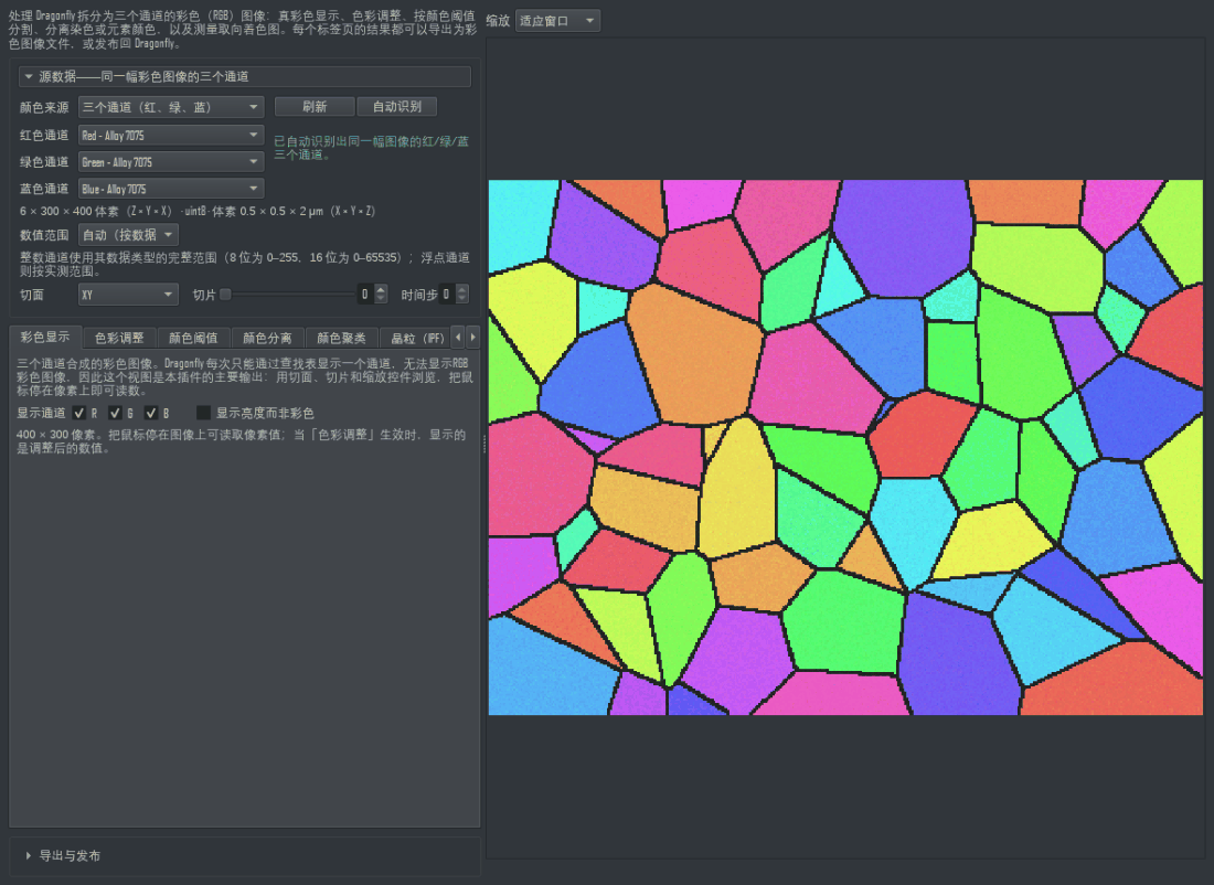
“彩色显示”页。Dragonfly 每次只能通过一个 LUT 显示单个通道，根本无法绘制 RGB 合成图——这一页就是那张合成图。

当「色彩调整」生效时，画面与悬停读数显示的都是调整后的数值，状态行会写明这一点。

可导出的图层：彩色图像，以及其亮度灰度图。

4. 标签页 2 — 色彩调整

色彩校正按固定顺序执行：白平衡 → 各通道色阶 → 伽马 → 亮度 → 对比度 → 饱和度 → 色相。顺序会影响结果——先做色阶还是先做伽马得到的像素并不相同——因此这里把顺序固定并写明，而不是取决于你先调哪个参数。

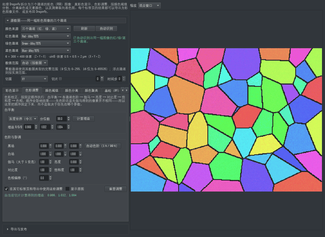
“色彩调整”页，这里点了一次白平衡。在您导出或发布之前，所有调整都只是显示变换。

• 白平衡：灰度世界令三通道均值相等；白块令某个高分位数（默认 99 %，这样单个亮点无法决定白场）相等；从选取的中性灰像素计算会等你点击一个应为中性灰的像素。三种方法都填入同样的三个增益框，之后仍可手动修改。
• 色阶：每个通道各有黑场与白场。自动色阶把它们设为当前切片的 1 % 与 99 % 分位点。
• 伽马大于 1 变亮。饱和度 0 为中性灰，1 为不变。色相偏移以度为单位旋转色环。

在其它标签页和导出中使用这些调整（默认勾选）正是本标签页影响整个面板的开关。取消勾选即可自由试验而不改变其它标签页的测量结果。显示原图可切回未处理的图像。

⚠ 白平衡和自动色阶都是从你当前看到的那一张切片计算的，而不是整个体数据。若整叠图像亮度存在漂移，请在两端各检查一次结果。

5. 标签页 3 — 颜色阈值

按三个分量的取值区间选取体素，与 ImageJ 的 Color Threshold 完全一致。颜色空间可选 RGB、HSV、CIE-Lab*、YCbCr，每个区间都以该空间自身的单位显示——色相为度，饱和度与明度为百分数，L* 为 0–100，a/b 约为 ±128，RGB 与 YCbCr 为 0–255。

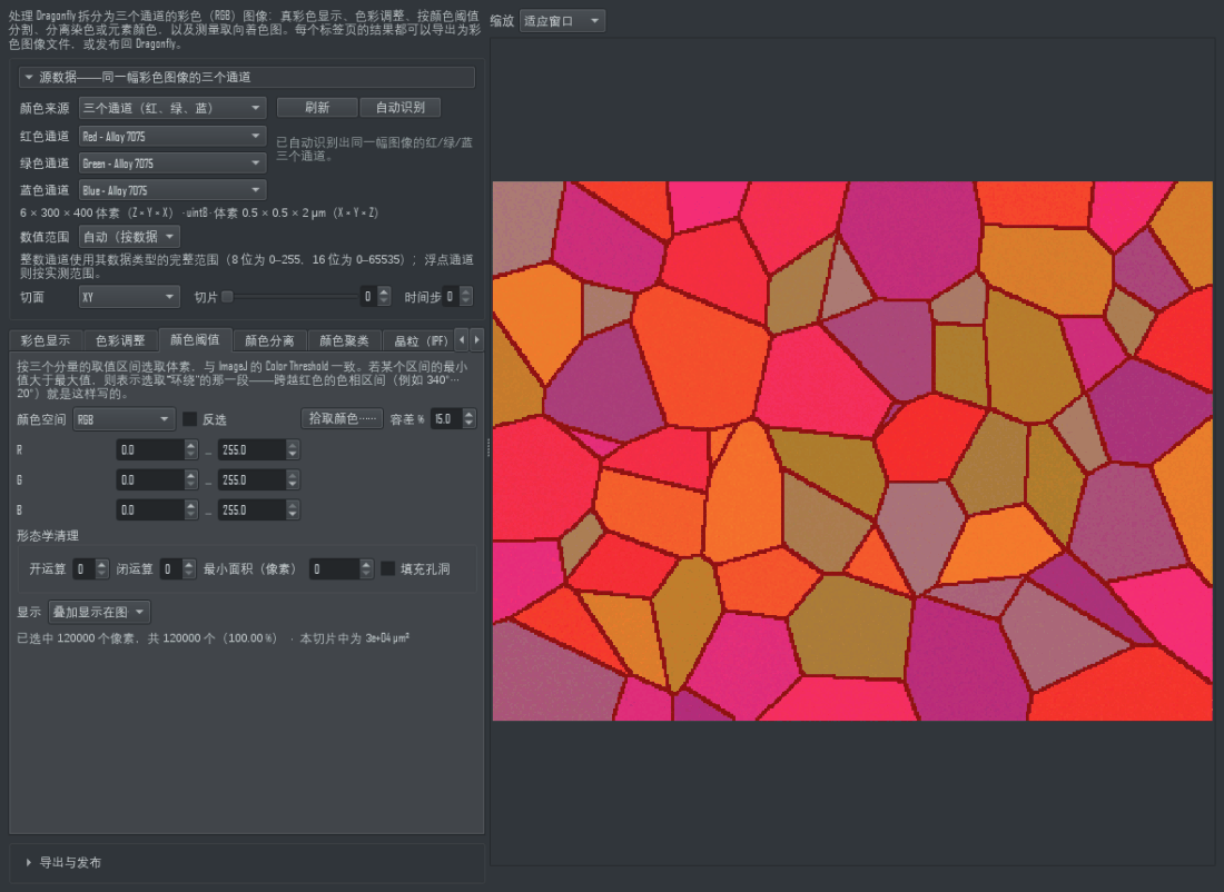
“颜色阈值”页。选择在您指定的颜色空间中定义；选中的掩膜可作为 ROI 发布，连通的各块也可作为 MultiROI 发布。

当某个区间的最小值大于最大值时，选取的是「环绕」的那一段。 跨越红色的色相区间（340°…20°）就是这样写的；因此不需要为每个分量单独设置反转开关。整体的反选复选框会把最终结果取反。

点击拾取颜色……后再点击图像，会按容差 %（相对于各分量完整范围的百分比）围绕该颜色设定三个区间。

形态学清理按顺序执行：开运算（去除杂点）、闭运算（连接细小孔洞）、最小连通面积（像素）、填充孔洞。状态行给出选中像素数、百分比，以及像素尺寸已知时的 µm² 面积。

可导出的图层，MultiROI 排在最前：选区作为 MultiROI（单个标签）、连通区域作为 MultiROI（每个区域一个标签，跨整叠切片统一编号，而不是每张切片重新开始；超过 65535 个区域会明确拒绝，而不是悄悄合并）、选区作为 ROI、选区内的图像，以及选区着色图（仅可导出）。

6. 标签页 4 — 颜色分离

两种拆分彩色图像的方式。

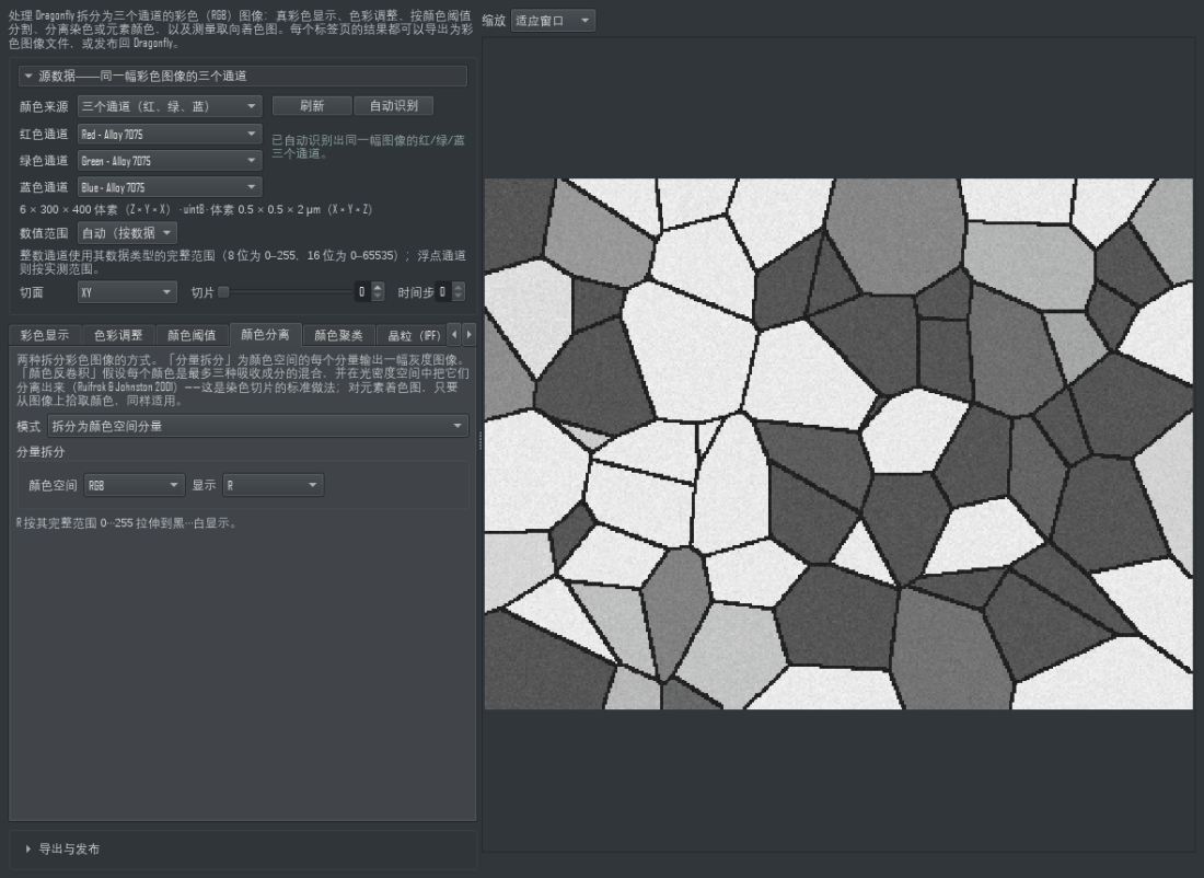
“颜色分离”页：可以拆成各分量，也可以做染色解混。负的分量会被如实报告而不是隐藏——正是这个比例告诉您染色向量选错了。

拆分为颜色空间分量

所选颜色空间的每个分量输出一幅灰度图像——色相、饱和度、明度；L、a、b*；等等。每幅图按该分量自身的完整范围拉伸到黑…白，并打印所用范围。

颜色反卷积

假设每个颜色是最多三种吸收成分的混合，并在光密度空间中把它们分离（Ruifrok & Johnston, 2001）——这是染色切片的标准做法。内置八种预设（H&E、H&E 2、H DAB、H AEC、Feulgen Light Green、Giemsa、Masson Trichrome、Alcian Blue & H）以及 RGB 与 CMY；每个向量都可手动修改，或通过点击只含某一种成分的像素来设定。第三个向量全为零时，会用前两者无法解释的残差成分代替。

⚠ 负值会被报告，而不会被隐藏。 某个成分系统性为负，说明这组向量并不适合这幅图像；把负值截断会把一个错误的预设变成一幅看起来很干净的图。面板会给出每个成分的均值、最大值和负值像素比例，比例超过 25 % 时给出警告。显示的图像是 10^(−含量)，因此颜色越深表示该成分越多，与 ImageJ 的显示方式一致。

7. 标签页 5 — 颜色聚类

找出图像中的颜色类别并发布为 MultiROI。一个类别是某种颜色的所有体素，无论位于何处——这与「晶粒」标签页的问题正好相反：同一颜色的两个分离区域，在这里是一个类别，在那里是两个晶粒。两个标签页并存，是因为这两个问题都会被问到。

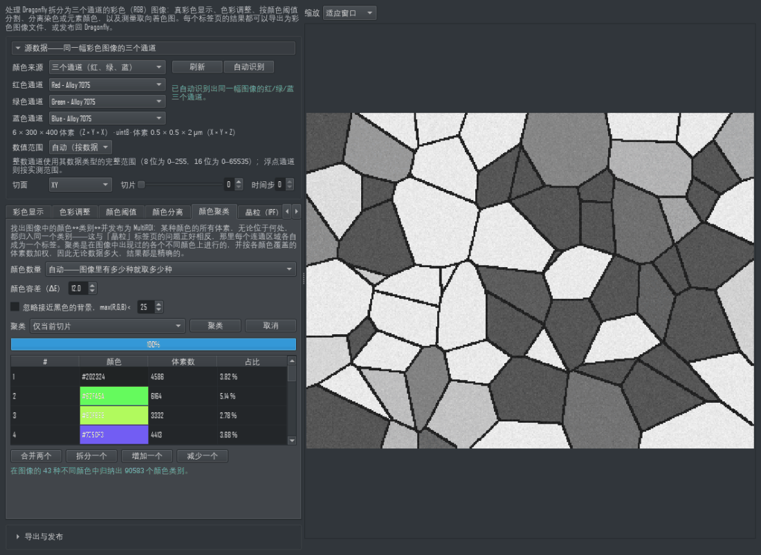
*“颜色聚类”页。一个类别是图像中任何位置上属于该颜色的所有体素，这与旁边的晶粒页回答的是不同的问题。*

本标签页取代了已停用的 Color Image to MultiROI 插件，其算法即来自该插件。

• 自动：由图像自身决定有多少种颜色——与已保留类别的 ΔE 色差在容差以内的颜色会并入该类别，而不是另起一类；最常见的颜色优先作为类别的种子。容差越小，类别越多。
• 指定数量（k）：用加权 k-means++ 求出正好 k 个类别。随机种子固定，因此同一幅图像、同一个 k 两次运行结果相同。
• 忽略接近黑色的背景：把 max(R,G,B) < 阈值以下的体素全部归为标签 0，使黑色底衬不进入任何类别。

聚类是在图像中出现过的各个不同颜色上进行的，并按各颜色覆盖的体素数加权，而不是逐体素计算，因此无论数据多大都既精确又快速。

随后可用表格进行修正：选中两行点合并两个，选中一行点拆分一个，或用增加一个 / 减少一个来拆分最分散的类别、合并最接近的一对。每次修改都会重新归类并重新精化，预览随之更新。

可导出的图层：颜色类别（MultiROI）（排在第一项，因此点「发布」默认发布它；每个标签都带有自身颜色与名称）、各类别以自身颜色显示的图像（仅可导出），以及图像本身。

8. 标签页 6 — 晶粒（IPF）

⚠ 这是基于颜色的分割，而非晶体学分割。 本插件不会从颜色反推取向，也不计算取向差。两个相邻且颜色恰好相近的晶粒会被合并。若需要真正的取向数据，请使用可读取 .ang / .ctf 文件的 EBSD 插件。

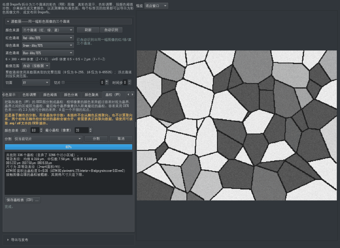
*“晶粒（IPF）”页。它是基于颜色的分割：不解码任何取向，也不计算取向差——页内的提示条已明确说明。*

相邻像素颜色差异超过容差（CIE76 色差：约 2.3 为刚可分辨的差异，8 是一个不错的起点）时视为晶界；晶界之间的区域即为晶粒；小于最小晶粒的区域被丢弃；最后每个晶界像素归入距离最近的晶粒，使晶界不会「吃掉」晶粒。

可选择仅当前切片或全部切片（三维）。结果框给出晶粒数量、等效直径的均值/中位数/标准差，以及 D10 / D50 / D90。单张切片给出二维等效圆直径 2·sqrt(面积/π)；真正的三维体给出等效球直径 (6·体积/π)^(1/3)。两者不可直接比较，因此每次都会写明用的是哪一种。

对于像素尺寸已知的二维图，还会给出 ASTM E112 面积法晶粒度 G，其中接触图像边缘的晶粒按半个计（该标准自身的约定），并在旁边打印计数与测量面积。

接触图像边缘的晶粒被截断，其测得尺寸只是下限。这一点每次都会写在结果框中。

保存晶粒表（CSV）为每个晶粒输出一行：体素数、尺寸、等效直径与平均颜色。可导出的图层：以平均颜色显示的晶粒、晶粒标签（发布为 MultiROI，每个标签使用该晶粒自身的平均颜色）、晶界（ROI），以及叠加晶界的图像。

9. 标签页 7 — 元素分布图（EDS）

以你列出的参考颜色（每行一个：名称、空格、#RRGGBB）测量元素着色合成图——EDS/SEM 分布图、物相图，或任何有已知色标的图像。从当前切片推荐会给出图中最常见且彼此可区分的颜色（每个都是相应体素的平均值，因此不会凭空造出图中没有的颜色）；点击图像添加则把光标下的颜色加入列表。

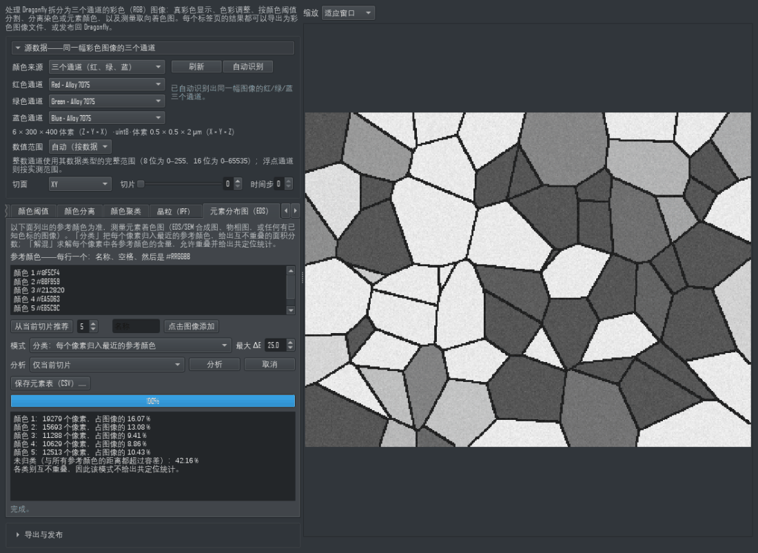
“元素分布（EDS）”页。在 RGB 图像上给出超过三个参考色时会被拒绝，而不是猜一个结果。

• 分类把每个像素归入 CIE76 色差最近的参考颜色。与所有参考颜色的距离都超过最大 ΔE 的像素保持未归类并计数。各类别互不重叠，因此该模式给出面积分数，并明确说明不适用共定位统计。
• 解混逐像素用最小二乘求解各参考颜色的含量。RGB 像素只有三个数值，因此超过三种参考颜色会被拒绝而不是硬猜。掩膜为含量超过掩膜阈值的像素，它们可以重叠，并对每一对给出共定位统计：交集、Jaccard 指数，以及两个方向的条件比例。

⚠ 解混使用的是普通最小二乘，负含量在显示时截断为 0，并非非负最小二乘。面板会报告发生截断的像素比例：比例过高说明这组参考颜色并不适合这幅图像。

保存元素表（CSV）输出每个元素的名称、参考颜色、像素数与比例。可导出的图层：元素标签（以参考颜色着色的 MultiROI）、分类后的图像、每个元素的掩膜，以及解混模式下每个元素的含量图。

10. 导出与发布

底部的一个导出栏服务于全部六个标签页。导出内容列出当前标签页能产出的结果；切片范围可选当前切片、指定范围或全部切片。

1. 在导出内容中选择要导出的图层。

2. 选择切片范围、输出文件夹和文件名前缀。

3. 选择格式：PNG 或 TIFF（无损）、BMP（不压缩）或 JPEG（有损，面板会提示）。TIFF 还可写成一个多页文件。

4. 导出图像文件……为每个切片写一个按编号命名的文件（编号位数可选），并在格式支持的位置写入像素尺寸。

5. 或点发布到 Dragonfly，把结果放回会话中。

发布产生什么取决于图层类型：彩色结果发布为三个通道，名称为 Red - <名称>、Green - <名称>、Blue - <名称>；灰度结果发布为一个通道；掩膜发布为 ROI；标签发布为携带各标签颜色的 MultiROI。它们都会沿用源数据的体素尺寸、方向与原点。

⚠ 发布必须选择「全部切片」。 新对象沿用源数据在空间中的位置，只发布部分切片会把结果画在错误的位置。选择子范围时会被拒绝并说明原因；此时请改为导出文件。

⚠ 分割结果发布为 MultiROI，而不是彩色图像。 所有做分割的标签页——颜色阈值、晶粒（IPF）、元素分布图——都把 MultiROI 图层放在第一项，因此点「发布」默认发布的就是它，且每个标签都带有自己的颜色和名称。分割结果的彩色渲染图（以平均颜色显示的晶粒、以参考颜色显示的元素、选区着色图、叠加晶界的图像）可以导出为图像文件，但故意不允许发布：发布它们只会得到三个 RGB 通道，其中的颜色是本插件画上去的，而不是分割结果本身。面板会说明这一点，并指向应当选择的 MultiROI 图层。

11. 本插件不做什么

• 不从 IPF 颜色反推晶体取向，也不计算取向差。
• 像素尺寸不可读时不给出面积或 ASTM 晶粒度，而是说明像素尺寸未知，不打印猜测值。
• 不做非负最小二乘，也不隐藏普通最小二乘与颜色反卷积产生的负值；正是这些数值告诉你参考颜色或染色向量选错了。
• CIE-Lab* 转换假设图像为 sRGB（D65 白点）。非 sRGB 的图像同样可以转换，只是不具备色度学意义。
• 色差采用 CIE76——即 Lab* 空间中的欧氏距离，对称且没有隐藏参数，但对高饱和度颜色并非感知均匀。

Part II English Manual

Contents

1. Introduction

2. The source: three channels of one image

3. Tab 1 — Color view

4. Tab 2 — Adjust

5. Tab 3 — Color threshold

6. Tab 4 — Separate

7. Tab 5 — Color clusters

8. Tab 6 — Grains (IPF)

9. Tab 7 — Element maps (EDS)

10. Export and publish

11. What this plugin does not do

1. Introduction

Dragonfly renders one channel at a time through a lookup table and cannot display an RGB composite. A colour image imported into Dragonfly therefore arrives as three grayscale channels — Red - ..., Green - ..., Blue - ... — that can only be looked at separately. This plugin puts them back together and does the colour work on top of them.

The panel has one source selector at the top (the three channels, the value range, the viewing plane, the slice and the time step), six tabs that all read that same source, and one export/publish footer that serves every tab.

Nothing in the session is created or modified until you press Publish. Everything else reads the three channels and writes files where you point it.

It runs in Dragonfly's own process on the numpy, scipy and Pillow Dragonfly already ships: no install, no internet, no GPU, no virtual environment.

2. The source: three channels of one image

The first box is filled with the first image channel whose title starts with "Red". The second and third are then filled with the Green and Blue channels whose names match that same image, so with two colour images open in the session Green - Sample 2 is never paired with Red - Sample 1.

• When no matching name exists, the first Green / Blue channel is used instead and the panel says the three may belong to another image.
• A title that merely contains the letters (Reduction) is not a red channel: whole words are matched, at the start of the title first, then at the end.
• Refresh re-reads the session after you publish something new; Auto-detect runs the matching again.

Value range decides how channel values become colour. Auto uses the data type's full range (0–255 for 8-bit, 0–65535 for 16-bit); float channels have no natural range and are measured instead. Measured uses each channel's own minimum and maximum. Custom applies one range to all three.

Plane chooses XY, XZ or YZ; the slider walks the remaining axis, and every tab — and the export — follows it. Time step picks the frame of a 4-D channel.

⚠ The three channels must have the same size. Three channels of different sizes are refused with their sizes printed, rather than being stretched to match.

3. Tab 1 — Color view

The RGB composite, at last. Use the plane, slice and Zoom controls to navigate; hover over a pixel to read its position, RGB, HSV and CIE-Lab* values. The R / G / B tick boxes switch a channel off (useful for seeing which channel carries a feature), and one more shows the luminance instead of the colour.

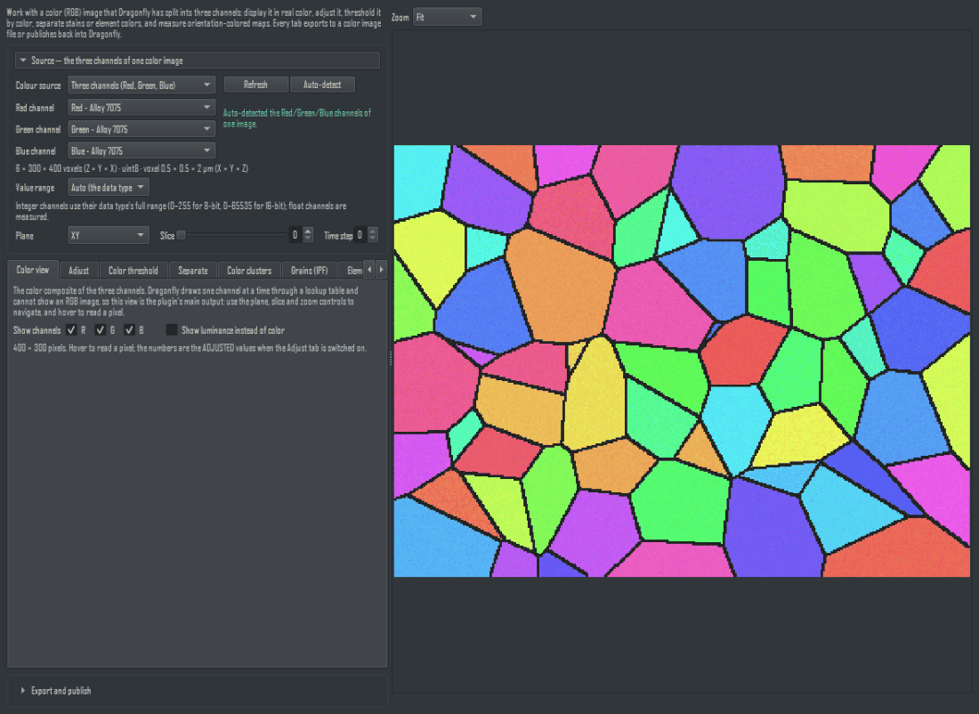
The Color view tab. Dragonfly renders one channel at a time through a LUT and cannot draw an RGB composite at all — this tab is that composite.

When the Adjust tab is switched on, both the picture and the hover readout show the adjusted values, and the status line says so.

Exportable layers: the colour image, and its luminance as a grayscale image.

4. Tab 2 — Adjust

Colour correction, applied in a fixed order: white balance, then per-channel levels, gamma, brightness, contrast, saturation and finally hue. The order changes the result — swapping levels and gamma gives different pixels — so it is pinned here rather than left to the order you happen to type in.

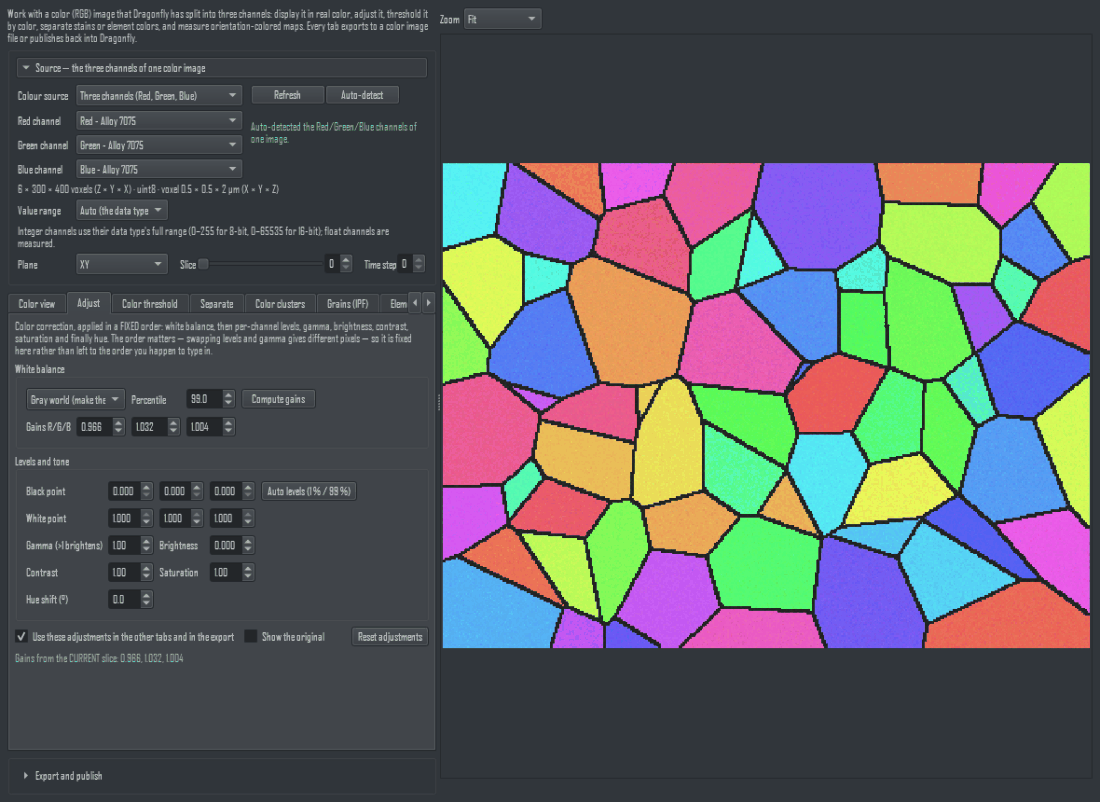
The Adjust tab after one click of white balance. Every adjustment is a display transform until you export or publish it.

• White balance: Gray world makes the three channel means equal; White patch equalises a bright percentile (99 % by default, so one hot pixel cannot set the white point); From a picked neutral pixel waits for you to click a pixel that should be neutral gray. All three fill the same three gain boxes, which you can then edit.
• Levels: a black and a white point per channel. Auto levels sets them to the 1 % and 99 % points of the slice you are looking at.
• Gamma above 1 brightens. Saturation 0 leaves a neutral gray, 1 is unchanged. Hue shift rotates the colour wheel in degrees.

Use these adjustments in the other tabs and in the export (on by default) is what makes this tab feed the whole panel. Untick it to experiment without changing what the other tabs measure. Show the original flips the preview back to the untouched image.

⚠ White balance and auto levels are computed from the slice you are LOOKING AT, not from the whole volume. On a stack whose brightness drifts, check the result at both ends.

5. Tab 3 — Color threshold

Select voxels whose colour falls inside three bands, exactly like ImageJ's Color Threshold. The colour space is RGB, HSV, CIE-Lab* or YCbCr, and each band is shown in that space's own units — hue in degrees, saturation and value in percent, L* 0–100, a/b about ±128, RGB and YCbCr 0–255.

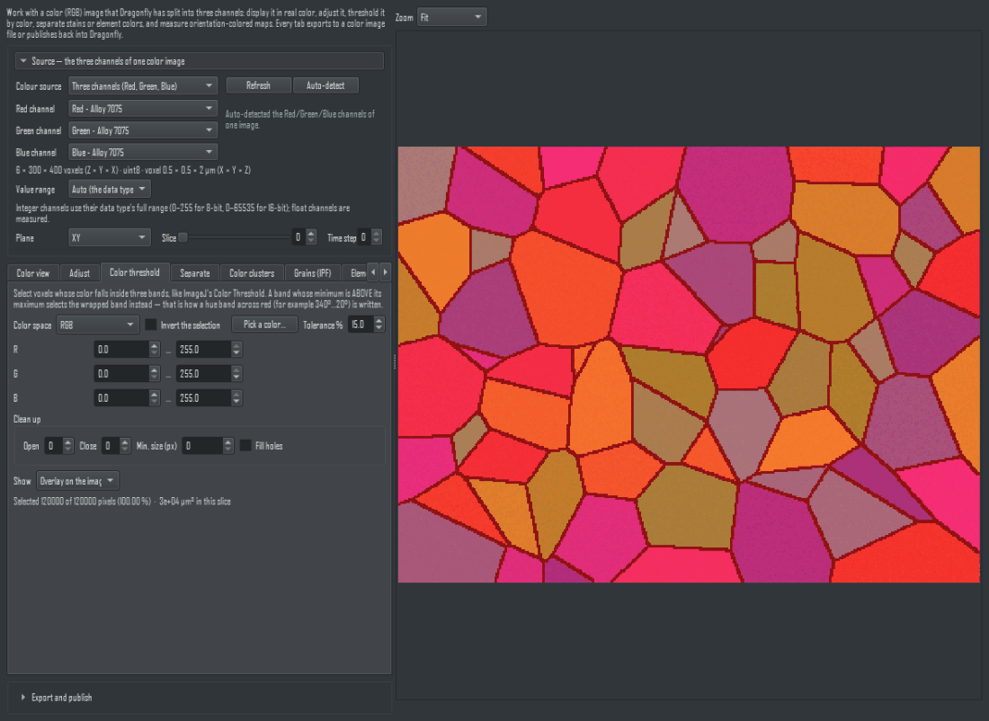
The Color threshold tab. The selection is defined in a colour space you choose, and the mask can be published as an ROI or the connected pieces as a MultiROI.

A band whose minimum is above its maximum selects the wrapped band. That is how a hue band across red — 340°…20° — is written; there is no separate invert box per band to get wrong. One Invert the selection box inverts the whole result.

Pick a colour… then clicking the image sets all three bands around that colour, as a percentage of each component's full range (the Tolerance % box).

Clean up applies, in order: opening (removes specks), closing (bridges pinholes), a minimum connected size in pixels, and hole filling. The status line gives the selected pixel count, the percentage, and the area in µm² when the pixel size is known.

Exportable layers, MultiROI first: the selection as a MultiROI (one label), the connected pieces as a MultiROI (one label each, numbered across the whole stack rather than restarted on every slice — more than 65535 pieces is refused rather than silently merged), the selection as an ROI, the image inside the selection, and the tinted overlay (export only).

6. Tab 4 — Separate

Two ways to take a colour image apart.

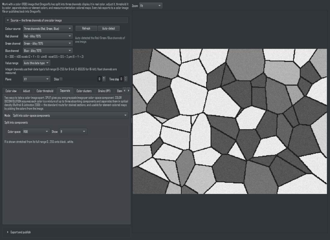
The Separate tab: split into components, or unmix stains. Negative amounts are reported rather than hidden — that fraction is how you learn the stain vectors are wrong.

Split into colour-space components

One grayscale image per component of the chosen space — hue, saturation, value; L, a, b*; and so on. Each is stretched from its own full range onto black…white, and the range used is printed.

Colour deconvolution

Assumes each colour is a mixture of up to three absorbing components and separates them in optical density (Ruifrok & Johnston, 2001) — the standard route for stained sections. Eight presets are provided (H&E, H&E 2, H DAB, H AEC, Feulgen Light Green, Giemsa, Masson Trichrome, Alcian Blue & H) plus RGB and CMY, and every vector can be edited or set by clicking a pixel that shows one component alone. An all-zero third vector is replaced by the residual that the first two do not explain.

⚠ Negative amounts are reported, not hidden. A systematically negative component means the vectors do not describe this image, and clipping it would turn a wrong preset into a clean-looking picture. The panel prints the mean, the maximum and the percentage of negative pixels for each component, and warns above 25 %. The displayed image is 10^(−amount), so dark means "much of this component", as ImageJ shows it.

7. Tab 5 — Color clusters

Finds the colour classes of the image and publishes them as a MultiROI. A class is every voxel of that colour, wherever it sits — which is the opposite question from the Grains tab: two separate regions of one colour are one class here and two grains there. Both tabs exist because both questions are asked.

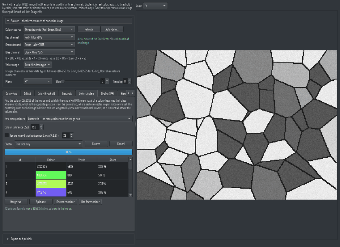
The Color clusters tab. A class is every voxel of that colour ANYWHERE in the image, which is a different question from the grain tab beside it.

This tab replaces the retired Color Image to MultiROI plugin, whose engine it is.

• Automatic decides how many colours the image has: colours within the ΔE tolerance of one already kept join it instead of starting their own, with the most common colours seeding the classes. Smaller tolerance, more classes.
• A fixed number (k) runs weighted k-means++ for exactly k classes. The seed is fixed, so the same image and the same k give the same answer twice.
• Ignore near-black background puts everything below max(R,G,B) < into label 0, which keeps a black surround out of the classes.

The clustering runs on the image's distinct colours weighted by voxel count, not on the voxels, so it is exact and quick however large the volume is.

The table then lets you correct it: select two rows and Merge two, one row and Split one, or use One more colour / One fewer colour to split the most spread-out class or merge the closest pair. Every edit re-assigns and re-refines, and the preview follows.

Exportable layers: the colour classes as a MultiROI (first, so Publish defaults to it — each label carries its own colour and a name), each class in its own colour (export only), and the image itself.

8. Tab 6 — Grains (IPF)

⚠ This is a colour segmentation, not a crystallographic one. No orientation is decoded from the colours and no misorientation is computed. Two touching grains that happen to be coloured alike will merge. For real orientation data use the EBSD plugins, which read .ang / .ctf files.

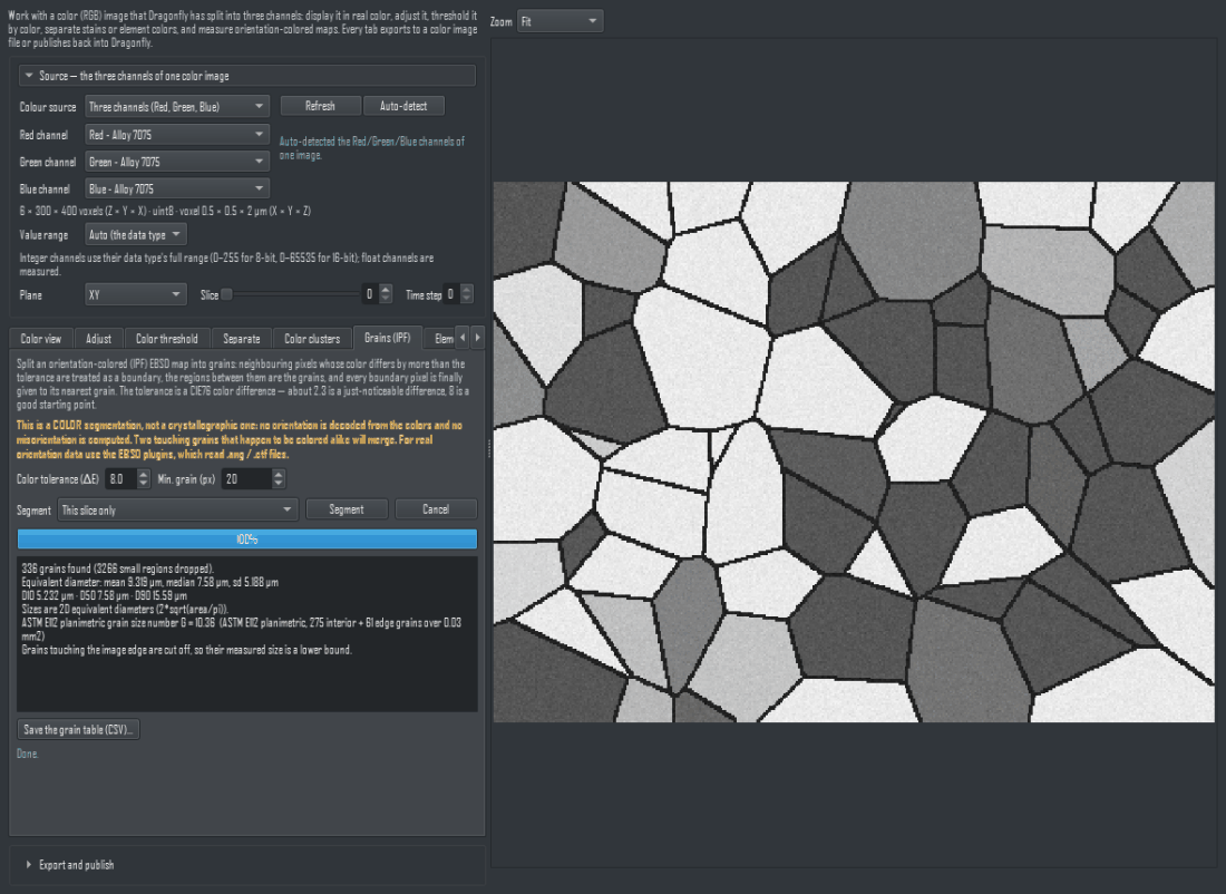
The Grains (IPF) tab. It is a COLOUR segmentation: it decodes no orientation and computes no misorientation, and the banner says so.

Neighbouring pixels whose colour differs by more than the tolerance (a CIE76 difference: about 2.3 is a just-noticeable difference, 8 is a good starting point) are treated as a boundary; the regions between them are the grains; regions smaller than Min. grain are dropped; and every boundary pixel is finally given to its nearest grain, so the boundary does not eat the grains.

Segment this slice only or all slices in 3-D. The results box gives the grain count, the mean / median / standard deviation of the equivalent diameter, and D10 / D50 / D90. A single slice gets a 2-D equivalent circle diameter, 2·sqrt(area/π); a real volume gets the sphere-equivalent (6·volume/π)^(1/3). The two are not comparable, so which one was used is always stated.

For a 2-D map with a known pixel size the ASTM E112 planimetric grain size number G is also given, counting grains that touch the image edge at half weight — the standard's own convention — with the counts and the measured area printed beside it.

Grains touching the image edge are cut off, so their measured size is a lower bound. This is stated in the results box every time.

Save the grain table (CSV) writes one row per grain: voxels, size, equivalent diameter and mean colour. Exportable layers: the grains in their mean colour, the grain labels (published as a MultiROI, each label coloured by that grain's own mean colour), the boundaries (an ROI), and the image with the boundaries drawn.

9. Tab 7 — Element maps (EDS)

Measures an element-coloured composite — an EDS/SEM map, a phase map, any image with a known colour key — against reference colours you list, one per line, as a name, a space and #RRGGBB. Suggest from this slice proposes the most common well-separated colours in the image (each one the mean of the voxels it stands for, so it never invents a colour that is not there); Add by clicking the image adds the colour under the cursor.

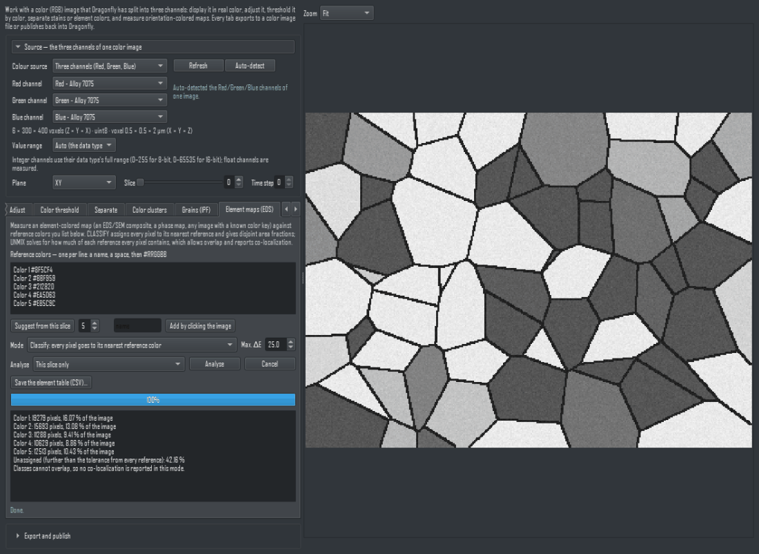
The Element maps (EDS) tab. More than three references on an RGB image is refused rather than guessed at.

• Classify puts every pixel in its nearest reference colour, measured as a CIE76 difference. A pixel further away than Max. ΔE from every reference is left unassigned and counted. The classes are disjoint, so this mode reports area fractions and says explicitly that no co-localization applies.
• Unmix solves, per pixel, how much of each reference it contains, by least squares. An RGB pixel carries three numbers, so more than three references is refused rather than guessed. Masks are then the pixels above the Mask threshold, they may overlap, and co-localization is reported for every pair: the intersection, the Jaccard index, and BOTH conditional fractions.

⚠ Unmixing is ordinary least squares with negative abundances clipped to zero for display — not non-negative least squares. The percentage of pixels where something had to be clipped is reported: a large value means the reference colours do not describe this image.

Save the element table (CSV) writes the name, reference colour, pixel count and fraction of every element. Exportable layers: the element labels (a MultiROI coloured by the reference colours), the classified image, one mask per element, and — in unmix mode — one abundance image per element.

10. Export and publish

One footer serves all six tabs. What to export lists whatever the tab you are on can produce; Slices is the current slice, a range, or all of them.

1. Pick the layer in What to export.

2. Choose the slices, the output folder and a file-name prefix.

3. Choose the format: PNG or TIFF (lossless), BMP (uncompressed) or JPEG (lossy — the panel says so). TIFF can also be written as one multi-page file.

4. Export image file(s)… writes one numbered file per slice — the digit width is yours to choose — with the pixel size written into the file where the format has a place for it.

5. Or Publish to Dragonfly to put the result back into the session.

What publishing produces depends on the layer: a colour result becomes three channels named Red - <name>, Green - <name> and Blue - <name>; a grayscale result one channel; a mask an ROI; labels a MultiROI carrying each label's colour. All of them inherit the source's voxel size, orientation and origin.

⚠ Publishing needs "All slices". The new object inherits the source's position in space, so publishing only part of the stack would draw the result in the wrong place. A sub-range is refused with that reason; export it to files instead.

⚠ A segmentation publishes as a MultiROI, not as a colour image. Every tab that segments — Color threshold, Grains (IPF), Element maps — lists its MultiROI layer FIRST, so Publish defaults to it, and each label carries its own colour and its own NAME. The coloured renderings of a segmentation (grains in their mean colour, elements in their reference colours, the tinted selection, the image with boundaries drawn) can be exported as image files but deliberately cannot be published: publishing one would add three RGB channels of colour this plugin painted on, instead of the segmentation itself. The panel says so and points at the MultiROI layer.

11. What this plugin does not do

• It does not decode a crystal orientation from an IPF colour, and it computes no misorientation.
• It does not report an area or an ASTM grain size when the pixel size cannot be read — it says the pixel size is unknown instead of printing a guess.
• It does not do non-negative least squares, and it does not hide the negative values that ordinary least squares and colour deconvolution produce; those numbers are how you tell that the reference colours or stain vectors are wrong.
• It assumes sRGB for the CIE-Lab* conversion (D65 white point). An image that is not sRGB still converts; it is simply not colorimetric.
• Colour differences are CIE76 — a plain distance in Lab*, symmetric and with no hidden parameters, but not perceptually uniform for saturated colours.