3D EBSD reconstruction(三维 EBSD 重建)
3D EBSD reconstruction - User Manual
Dragonfly Prototype Apps · 3D EBSD reconstruction...
版本 Version 1.0 · 2026-09-01
第一部分 中文手册
目录
1. 简介
2. 本插件固定的约定
3. 标签页 1 — 载入
4. 标签页 2 — 清理
5. 标签页 3 — 对齐
6. 标签页 4 — 分割
7. 标签页 5 — 测量
8. 标签页 6 — 发布
9. 本插件不做的事
1. 简介
电子背散射衍射(EBSD)在样品表面的每一个点上测量一个晶体取向。连续切片把这一测量逐层重复,本插件把由此得到的序列重建为三维晶粒结构。
六个标签页本身就是工作流程,按顺序排列。所有标签页从一开始就是打开的,您可以先阅读并设置每一页再运行;尚不具备输入的步骤会在它自己的按钮处拒绝执行,并告诉您应先运行哪一步。“载入”页上的按当前设置执行全部步骤按钮,会用每一页当时的设置无人值守地跑完整个流程。
在最后一个标签页按下发布之前,插件不会在您的会话中创建或修改任何对象。
为什么这不是简单的颜色分割。 反极图(IPF)是把取向渲染成颜色,两个不同的取向可能被渲染成几乎相同的颜色。本插件直接在取向本身上做分割——计算相邻体素之间的取向差,并考虑晶体对称性——因此在颜色上看起来是一个晶粒的孪晶,在这里仍然是两个晶粒。如果您手里只有一张 IPF 的彩色图片而没有取向数据,请使用《彩色图像处理》插件,那里也明确说明它不解码任何取向。
2. 本插件固定的约定
以下每一条都是 EBSD 工作中有据可查的错误来源,因此都在数据入口处一次性固定,并在此说明。
- 欧拉角采用 Bunge(ZXZ)约定。
.ang文件以弧度存储,.ctf文件以角度存储;读取时即完成换算,后续步骤无需再关心来源。 - 四元数为 (w, x, y, z),单位长度,且 w ≥ 0,使一个旋转只有一种表示。
- 报告的是取向差(disorientation):在所有对称等价表示中取最小角度。对于立方—立方,该角度不可能超过 62.8 度,这是最简单有效的合理性检验。
- 面板中的长度单位一律为微米。 发布结果时会换算为米(Dragonfly 的存储单位),因此在 Dragonfly 中测得的数值与“测量”页一致。
3. 标签页 1 — 载入
顶部可选择三种数据来源:
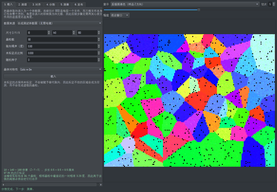
标签页 1「载入」。文件自身的约定会被读取并显示出来,不做任何假设。
- 连续切片文件夹(
.ang/.ctf)。文件按自然顺序排序,因此slice_2排在slice_10之前;普通的字母排序会把连续切片排错。切片间距需要您填写,因为单层文件本身并不记录它。 - 单个三维文件(HDF5、
.h5ebsd、DREAM.3D)。候选数据集列表按形状构建——末维为 3(欧拉角)或 4(四元数)——而不是按名称,并由您选择,因为仅凭名称无法确定数据集的内容。若文件存储的是角度,请勾选相应选项。 - 合成测试体数据,便于在没有电镜数据时熟悉整个流程。它会报告自己真实的晶粒数,以及相邻晶粒中最接近的一对取向差——这是任何阈值都必须遵守的上界。
请在载入前设置晶体对称性。网格形状由点的坐标推导,而不是取自文件头:被截断的导出文件其文件头仍然声称完整尺寸,若加以信任会把数据重排成无意义的结果。
未标定的点保持未标定。 它们不会被赋予替代取向,因此标定不佳的区域会成为空洞,而不会变成虚假的晶粒。
4. 标签页 2 — 清理
剔除电镜无法可靠标定的点:置信度(.ang 中的 CI、.ctf 中的 MAD)低于阈值的点,或物相为 0 的点。若数据不含相应的列,相关控件会被禁用并明确说明原因。
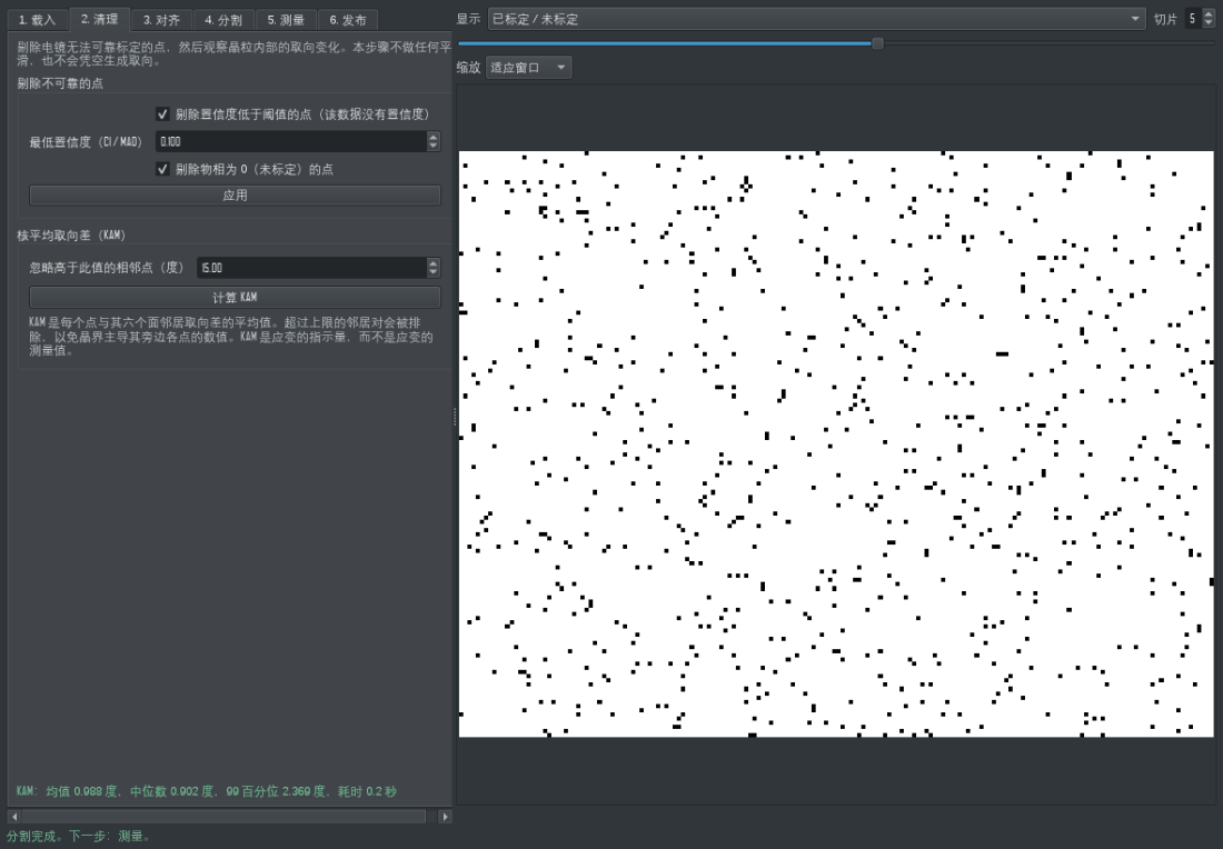
标签页 2「清理」。每一步清理都会报告改动了多少个点,因此过度的设置是看得见的。
清理始终从载入时的数据重新开始,因此阈值设置得过高时可以直接调低,而不必重新载入。
核平均取向差(KAM) 是每个点与其六个面邻居取向差的平均值。超过上限的邻居对会被排除而不是截断,以免晶界主导其旁边各点的数值。
KAM 是应变的指示量,而不是应变的测量值。它随储存的位错密度上升,但其绝对数值取决于步长和标定的角分辨率,因此只能在同一套数据内部比较,不能跨设备比较。
执行清理或计算 KAM 会清除已识别的晶粒,因为它们与所依据的数据已不再一致。
5. 标签页 3 — 对齐
连续切片会发生漂移。未对齐的序列会把一个晶粒变成一串阶梯状的独立晶粒,因此即使漂移看起来很小,也值得在分割之前运行本步骤。
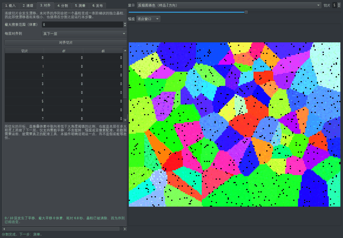
标签页 3「对齐」。
所优化的目标,是重叠体素中取向差低于大角度阈值的比例——也就是本层在多大程度上延续了下一层。这才是真正重要的量,而不是在彩色渲染图上做图像相关。
仅支持整数平移:不含旋转、缩放或亚像素配准。 若数据需要这些,就需要真正的配准工具,本插件明确说明这一点,而不是假装能够胜任。每一层实际施加的平移量都会列出,便于检查。
6. 标签页 4 — 分割
当相邻两个体素的取向差超过阈值时,它们之间的面即为晶界;剩下的连通区域就是晶粒。本步骤在三维中运行,因此一个晶粒是贯穿整个序列的单一对象,而不是每层各自独立的区域。
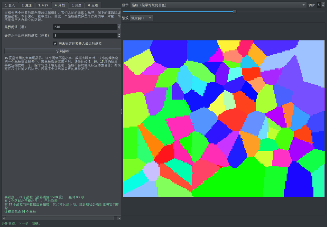
*标签页 4「分割」。晶粒是从取向中找出来的,而不是从图片中;阈值的敏感性会如实给出,而不是藏起来。*
阈值不是小事。 15 度是常用的大角度晶界,但数据有噪声时,过小的阈值会把一个晶粒拆成很多个:在取向噪声为 1 度的模型上,2 度阈值给出一千多个晶粒,而 5 度与 15 度都给出约 35 个。若晶粒数看起来不对,请先比较 5、10、15 度的结果,再决定相信哪一个。
- 丢弃小于指定体积的晶粒,用于去掉噪声产生的碎点。
- 把未标定体素并入最近的晶粒是常用的晶粒膨胀清理,使晶粒内部的小片未标定区域不会形成空洞。它在尺寸过滤之后执行,因此不会让已被丢弃的晶粒复活。
除非勾选该选项,晶粒不会跨越未标定体素合并。
7. 标签页 5 — 测量
每个晶粒:体素数、体积,以及等效直径——与该晶粒体积相同的球体的直径。整个体数据:均值、中位数以及 D10 / D50 / D90。
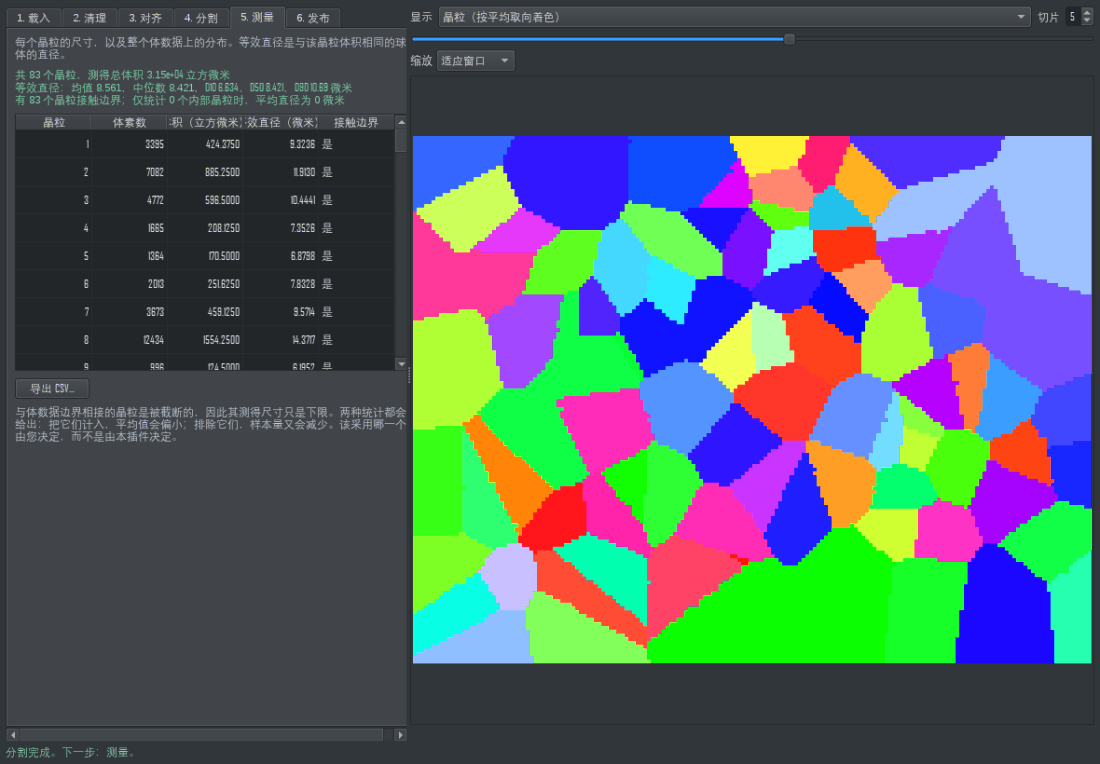
标签页 5「测量」。
与体数据边界相接的晶粒是被截断的,因此其测得尺寸只是下限。两种统计都会给出:把它们计入,平均值会偏小;排除它们,样本量又会减少。该采用哪一个由您决定,而不是由本插件决定。
导出 CSV 会写出全部晶粒,并包含每个晶粒以四元数表示的平均取向。一组旋转的平均取向按外积之和的主特征向量计算,该结果与每个四元数任意的符号无关。
8. 标签页 6 — 发布
晶粒以 MultiROI 的形式加入,因为在 Dragonfly 中分割结果就应当是 MultiROI:每个晶粒一个标签,以其尺寸命名,并按其自身的平均取向着色。
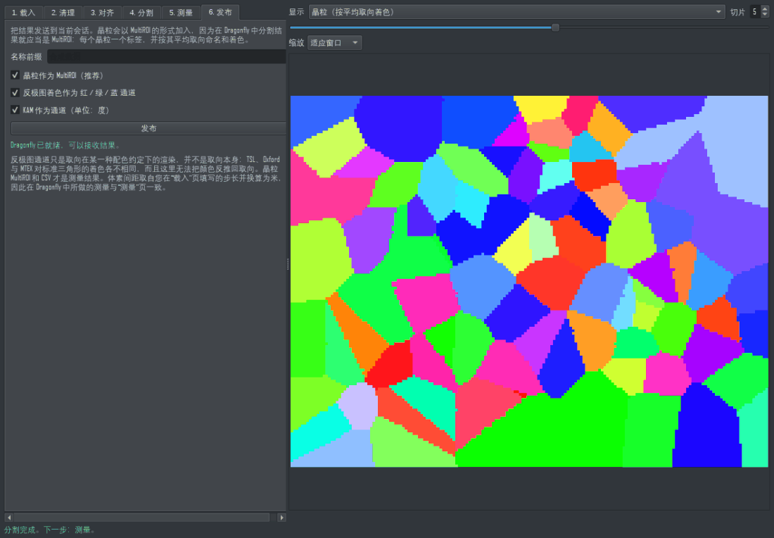
标签页 6「发布」。分割结果以 MultiROI 发布;IPF 与 KAM 通道是可选附加项,并被明确标注为“渲染结果”。
还可以选择把反极图着色作为红/绿/蓝三个通道加入,把 KAM 作为以度为单位的通道加入。
反极图通道只是渲染,不是数据。 TSL、Oxford 与 MTEX 对标准三角形的着色各不相同,因此本插件与厂商软件的颜色无法逐像素比较,而且这里无法把颜色反推回取向。晶粒 MultiROI 和 CSV 才是测量结果。
体素间距取自您在“载入”页填写的步长并换算为米。若某个对象未能成功设置间距,面板会明确说明,而不是留给您在测量时才发现。
9. 本插件不做的事
- 不做衍射花样标定。 它从厂商软件已经标定好的取向开始。
- 不做亚像素或含旋转的切片配准。 仅支持整数平移。
- 不计算 HR-EBSD 弹性应变,KAM 也不能替代它。
- 不按 Σ 值识别孪晶或特殊晶界,也不生成取向差分布函数或极图。
- 不为非立方晶系着色反极图。 六方对称支持取向差与分割,但反极图着色会拒绝,而不是猜一个约定。
- 不把颜色反推回取向,这也是为什么单纯一张 IPF 图片永远无法作为本插件的输入。
Part II English Manual
Contents
1. Introduction
2. Conventions this plugin fixes
3. Tab 1 - Load
4. Tab 2 - Clean
5. Tab 3 - Align
6. Tab 4 - Segment
7. Tab 5 - Measure
8. Tab 6 - Publish
9. What this plugin does not do
1. Introduction
Electron backscatter diffraction measures a crystal orientation at every point of a surface. Serial sectioning repeats that measurement slice by slice, and this plugin turns the resulting stack into a three-dimensional grain structure.
The six tabs are the workflow itself, in order. Every tab is open from the start, so you can read and set them all before running anything; a step whose input does not exist yet refuses at its own button and names the step you have to run first. One button on the Load tab, Execute All Steps with Current Settings, runs the whole workflow unattended with the settings each tab shows at that moment.
Nothing is created or modified in your session until you press Publish on the last tab.
Why this is not just a colour segmentation. An IPF map is orientation rendered as colour, and two different orientations can be rendered in nearly the same colour. This plugin segments on the orientations themselves - the disorientation between neighbouring voxels, with crystal symmetry taken into account - so a twin that looks like one grain in colour is still two grains here. If you only have a colour picture of an IPF map and not the orientation data, use Color Image Processing instead, which says plainly that it decodes no orientation.
2. Conventions this plugin fixes
Every one of these is a documented source of wrong answers in EBSD work, so each is fixed once, at the boundary, and stated here.
- Euler angles are Bunge (ZXZ).
.angfiles store them in radians and.ctffiles in degrees; the readers convert, so nothing downstream has to remember which file it came from. - Quaternions are (w, x, y, z), unit length, with w >= 0, so a rotation has exactly one representation.
- What is reported is the disorientation: the smallest angle over all symmetry-equivalent representations. For cubic-cubic that can never exceed 62.8 degrees, which is the cheapest sanity check there is.
- Lengths are micrometres throughout the panel. When results are published, the spacing is converted to metres, which is what Dragonfly stores, so measurements made in Dragonfly agree with the Measure tab.
3. Tab 1 - Load
Three sources, chosen at the top:
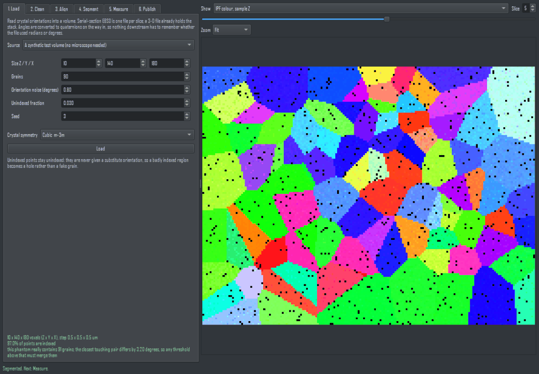
Tab 1, Load. The file's own conventions are read and shown; nothing is assumed.
- A folder of serial sections (
.ang/.ctf). Files are sorted naturally, soslice_2comes beforeslice_10; plain alphabetical sorting gets serial sections wrong. You give the slice spacing, because no single-slice file records it. - One 3-D file (HDF5,
.h5ebsd, DREAM.3D). The dataset list is built by shape - a trailing axis of 3 (Euler) or 4 (quaternion) - not by name, and you choose from it, because a name alone does not prove what a dataset holds. Tick the box if the file stores degrees. - A synthetic test volume, so the workflow can be tried without a microscope. It reports its own true grain count and the closest touching pair of orientations, which is the bound any threshold has to respect.
Set the crystal symmetry before loading. Grid shape is derived from the point coordinates, not from the header: a truncated export still claims its full size in the header, and trusting that reshapes the data into nonsense.
Unindexed points stay unindexed. They are never given a substitute orientation, so a badly indexed region becomes a hole rather than a fake grain.
4. Tab 2 - Clean
Drop points the microscope could not index reliably: below a confidence (CI in .ang, MAD in .ctf) or carrying phase 0. The controls are disabled, and say so, when the dataset carries no such column.
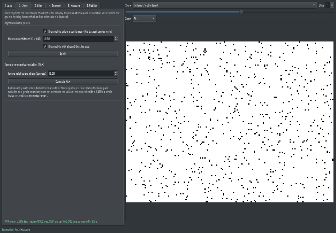
Tab 2, Clean. Every cleaning step reports how many points it changed, so a destructive setting is visible.
Cleaning always restarts from the data as loaded, so a threshold that was set too high can simply be lowered again without reloading.
Kernel average misorientation (KAM) is each point's mean disorientation to its six face neighbours. Pairs above the ceiling are excluded, not clipped, so a grain boundary does not dominate the value of the points beside it.
KAM is a strain indicator, not a strain measurement. It rises with stored dislocation content, but its absolute value depends on the step size and on the angular resolution of the indexing, so numbers are comparable within one dataset and not across instruments.
Running Clean or computing KAM clears any grains already found, because they would no longer match the data they came from.
5. Tab 3 - Align
Serial sectioning drifts. An unaligned stack turns one grain into a staircase of separate grains, so this is worth running before Segment even when the drift looks small.
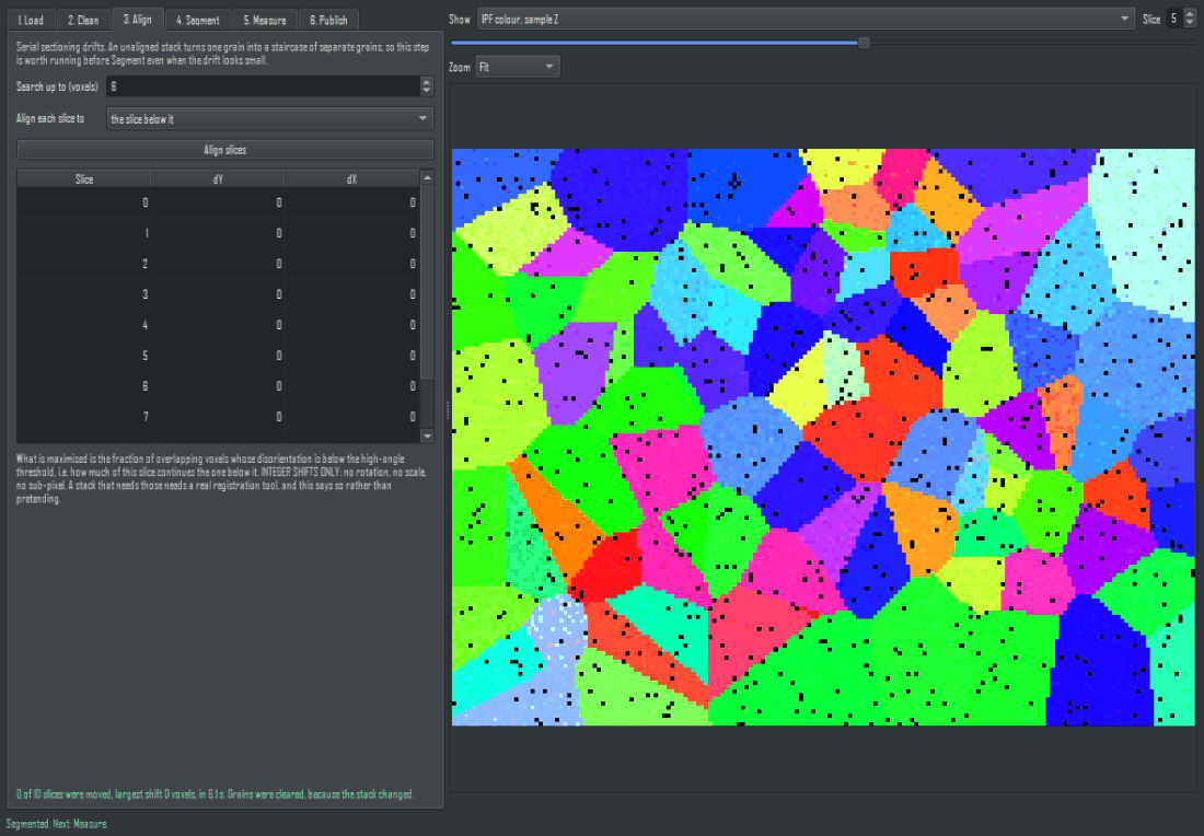
Tab 3, Align.
What is maximised is the fraction of overlapping voxels whose disorientation is below the high-angle threshold - that is, how much of this slice continues the one below it. That is the thing that actually matters, rather than an image correlation on a colour rendering.
Integer shifts only: no rotation, no scale, no sub-pixel. A stack that needs those needs a real registration tool, and this says so rather than pretending. The shift applied to every slice is listed so you can see what happened.
6. Tab 4 - Segment
A face between two neighbouring voxels is a boundary when their disorientation exceeds the threshold; the grains are the connected regions that remain. This runs in 3-D, so a grain is one object through the whole stack rather than a separate region on every slice.
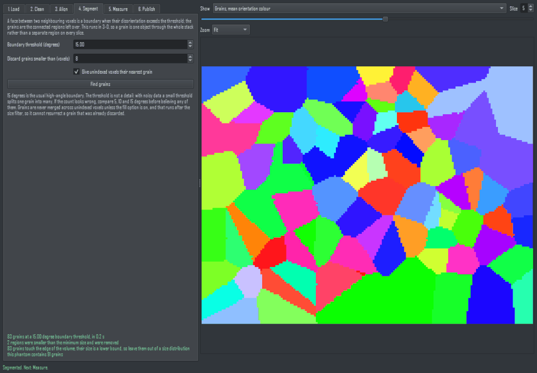
Tab 4, Segment. Grains are found from ORIENTATIONS, not from a picture; the threshold's sensitivity is published rather than hidden.
The threshold is not a detail. 15 degrees is the usual high-angle boundary, but with noisy data a small threshold splits one grain into many: on a phantom with 1 degree of orientation noise, 2 degrees gave over a thousand grains where 5 and 15 degrees both gave about 35. If the count looks wrong, compare 5, 10 and 15 degrees before believing any of them.
- Discard grains smaller than removes specks left by noise.
- Give unindexed voxels their nearest grain is the usual grain dilation clean-up, so small unindexed patches inside a grain do not punch holes in it. It runs after the size filter, so it cannot resurrect a grain that was already discarded.
Grains are never merged across unindexed voxels unless that option is on.
7. Tab 5 - Measure
Per grain: voxel count, volume, and equivalent diameter - the diameter of the sphere with the same volume. Over the volume: mean, median and D10 / D50 / D90.
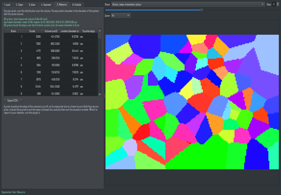
Tab 5, Measure.
A grain touching the edge of the volume is cut off, so its measured size is a lower bound. Both figures are given: include those grains and the mean is biased low, exclude them and the sample is smaller. Which to report is your decision, not this plugin's.
Export CSV writes every grain, including its mean orientation as a quaternion. The mean orientation of a set of rotations is computed as the dominant eigenvector of the summed outer product, which is invariant to each quaternion's arbitrary sign.
8. Tab 6 - Publish
The grains go in as a MultiROI, which is what a segmentation is in Dragonfly: one label per grain, named with its size and coloured by its own mean orientation.
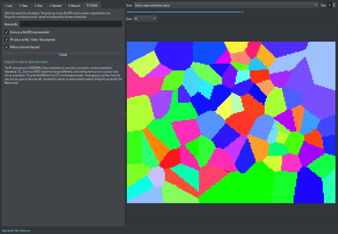
Tab 6, Publish. A segmentation publishes as a MultiROI; the IPF and KAM channels are optional extras, labelled as renderings.
Optionally the IPF colouring goes in as three Red / Green / Blue channels, and KAM as a channel in degrees.
The IPF channels are a rendering, not data. TSL, Oxford and MTEX shade the standard triangle differently, so colours from this plugin and from a vendor package are not comparable pixel for pixel, and nothing here can turn a colour back into an orientation. The grain MultiROI and the CSV are the measurement.
Voxel spacing is written from the step size you gave on the Load tab, converted to metres. If it could not be set on some object, the panel says so instead of leaving you to discover it by measuring.
9. What this plugin does not do
- It does not index diffraction patterns. It starts from orientations a vendor package has already indexed.
- It does not do sub-pixel or rotational slice registration. Integer shifts only.
- It does not compute HR-EBSD elastic strain, and KAM is not a substitute for it.
- It does not identify twins or special boundaries by their sigma value, and does not produce a misorientation distribution function or a pole figure.
- It does not colour non-cubic IPF maps. Hexagonal symmetry is supported for misorientation and segmentation, but the IPF colouring refuses rather than guessing a convention.
- It does not invert a colour back into an orientation, which is why an IPF picture alone can never be used as input here.