Optical Metallography 3D（金相三维重建）

Optical Metallography 3D - User Manual

Dragonfly Prototype Apps · Optical Metallography 3D...

版本 Version 1.9 · 2026-09-07

第一部分 中文手册

目录

1. 简介

2. 标签页 1 — 数据源

3. 标签页 2 — 切片对齐（可选）

4. 标签页 3 — 预处理

5. 标签页 4 — 初步晶界

6. 标签页 5 — 晶粒

7. 标签页 6 — 三维连接

8. 标签页 7 — 插值（可选）

9. 标签页 8 — 测量与发布

10. 如何判断您的序列究竟能不能做三维重建

11. 本插件不做的事

1. 简介

腐蚀后的金相显微照片上，晶界表现为深色的线，而每个晶粒内部看起来完全一样。全部信息都在晶界网络里。本插件逐层分割这个网络，再把结果连接成三维晶粒。

八个标签页本身就是工作流程。每一步只有在上一步产生结果之后才会开放，因此不会不小心跳过步骤。第七页“插值”是可选的，而且它被特意放在测量之前：如果您运行了它，第八页就在插值体上测量并发布；如果您跳过它、或者丢弃它的结果，第八页测量的就是切片被切出来时的原样。在您按下某个发布按钮之前——标签页 2 可选的对齐图像，或标签页 8 的结果——插件不会在您的会话中创建任何对象。

为什么这既不是 EBSD 插件，也不是颜色分割。 在 EBSD 图中，晶粒的身份是每个像素上测得的取向。而这里根本没有取向，晶粒内部也没有可区分的颜色：在参考数据上实测，不同晶粒内部之间的 CIE76 色差只有 7.2（属于噪声），而基体与晶界之间是 49.5。因此任何基于内部颜色做聚类或区域生长的方法，在这里根本无法区分晶粒。如果您有取向数据，请用《三维 EBSD 重建》；如果只有一张 IPF 的彩色图片，《彩色图像处理》已明确说明它不解码任何取向。

在图像区域中： 滚动鼠标滚轮可逐层浏览切片；按住鼠标中键拖动可缩放（光标下的那一点保持不动）；同时按住左键和右键拖动可平移。左边缘的刻度尺以图像像素为单位，并随缩放自动改变刻度；图像下方的一行会告诉您当前屏幕上显示了多大的范围——本插件里所有参数都以像素为单位，选参数时正需要这个数字。切片号旁边还会给出 Dragonfly 自己的视图为这一层显示的切片号（Dragonfly 可能从另一端开始计数）；当 Dragonfly 当前的 2D 视图把图像镜像显示时，预览也会同样镜像，两边看到的是同一幅、同一朝向的图像。在 Dragonfly 中显示 按钮会把 Dragonfly 当前的 2D 视图切换到这里正在看的切片。这两项都在每次预览重绘时从实际视图读取；如果该视图不是这幅图像的 XY 切片视图，面板会明确说明，按钮也会禁用。

「数据源」页的一键执行全部步骤（按当前设置）会无人值守地跑完整个流程：加载 → 对齐 → 提交预处理与边界参数 → 晶粒分割 → 三维连接 → 发布，每一步都使用你按下按钮那一刻各自页签上显示的设置，因此可以按下之后离开，回来再看结果。插值与网格化默认关闭（它们最昂贵），对齐默认开启（与「对齐」页自身的自动应用一致）；三者都是按钮旁的复选框，被跳过的步骤会写进运行日志。所有页签始终可以打开和修改参数，正是为了能在运行之前逐页检查：某一步所需的输入尚不存在时，按下它自己的按钮会给出提示，说明缺的是哪一步。

2. 标签页 1 — 数据源

选择已经导入 Dragonfly 的图像。体素尺寸取自通道本身，因此只要您在 Dragonfly 中标定过一次，本插件中的所有长度都是微米。若 Dragonfly 未提供体素尺寸，面板会明确说明，并把所有长度标注为“体素”，而不是悄悄假装有标定。

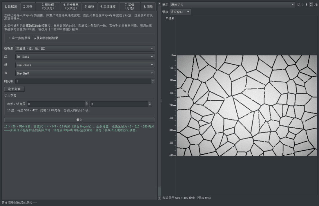
“数据源”页：选择通道与切片范围；运行所需的内存与时间会在您动手之前就给出。

• 单通道：用于灰度图，或彩色图的某一个通道。
• 三通道：用于 Dragonfly 把彩色图拆成的 红 / 绿 / 蓝。它们按名称配对：先找首个前导词为 “Red” 的标题，再取名称与之匹配的 Green 和 Blue。若按位置配对，只要同时打开两幅彩色图，就会把 “Green - Sample 2” 配到 “Red - Sample 1” 上。

三个通道按标准亮度权重合成。切片范围便于先在一部分数据上调参数；所需内存与预计耗时会在您确认之前先打印出来，因为参考数据是 2.07 亿个体素。

3. 标签页 2 — 切片对齐（可选）

⚠ Dragonfly 本身就带有功能完整的 Slice Registration（切片配准），而且它比这里的更强。在 Data Properties and Settings 面板中右键点击您的数据集，选择 Slice Registration 即可打开：它提供增强相关系数（ECC）、基于特征、互信息、SSD、光流、模板匹配等多种算法，除平移外还支持旋转，带漂移补偿，可逐层手工调整，变换模板还能保存复用。只要各层存在旋转、变形或偏移较大，或者配准本身就是您要的结果，请使用它。

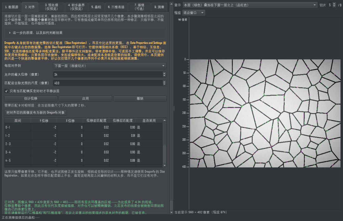
“对齐”页：顶部标明 Dragonfly 自带的 Slice Registration；下方是每一对相邻层实测的位移，以及位移前后的匹配度。

本标签页有意只做最小而有用的那一种修正，好让仅仅错开几个像素的序列不必离开本面板就能继续测量：每层一次整像素平移。不做旋转、不做缩放、不做亚像素平移、不做任何插值。这一步是可选的——如果各层本来就叠得很齐，跳过即可。

1. 把图像上方的显示切换为 本层（绿色）叠加在下面一层之上（品红色），拖动滑块逐层查看。两层一致的地方，颜色会相互抵消成灰色；没有对齐的地方会出现彩色镶边，镶边多宽，误差就有多大。

2. 点击 估计位移。相邻两层之间用互相关做匹配，表格随之填出：找到的位移，以及位移前后两层的匹配度。此时数据还没有被移动。

3. 阅读表格。只有当“位移后匹配度”明显高于“位移前匹配度”时，这次平移才值得采用；是否采用一列会告诉您结果。

4. 点击 应用。各层被平移，并裁剪到所有层共同覆盖的矩形——面板会报告这样做损失了多少视场。

5. 撤销 随时可以把完整视场精确地恢复回来。

6. 可选：把对齐后的图像发布为新的 Dragonfly 对象 会把对齐后的各层作为一个新的图像通道送进您的会话。本插件后面的步骤并不需要它——它是为了让您能用 Dragonfly 自己的工具处理对齐后的序列，或者把它保存下来。发布出去的图像与原始图像尺寸、位置完全一致，因此会与原图重合；每层因平移而从画面外移进来的那一条保持为 0，面板会告诉您“在所有层上都有真实数据”的矩形范围。如果您只想要那个矩形，请在 Dragonfly 里裁剪——Dragonfly 的裁剪会把原点一起移动过去，这正是本插件不直接给出已裁剪对象的原因。

7. “估计位移后立刻自动应用”默认勾选：按“估计位移”会在测出位移后直接平移整叠图像，一步完成，“撤销”仍可精确还原；取消勾选则先看表格，再自行按“应用”。该勾选状态会被记住。

为什么只做整像素。 后面每一步阈值处理的，都是那些又细又暗的晶界线，而它们是腐蚀金相照片里唯一的信息。亚像素平移或旋转都必须重采样，而重采样恰恰会模糊这些线。整像素平移只是搬动数据，不改变任何灰度值；它同时可以被精确还原，这正是为什么在对齐后的数据上测出的晶粒，仍然能发布到原始图像自己的体素位置上。

先对齐，再对样品下结论。 如果某一对相邻层在平移之后匹配度依然很低，那确实是断裂：这两层之间磨掉的材料太多，任何配准都救不回来。但仅仅是发生了平移的层间，看起来和断裂一模一样——因为它的晶粒不再重叠。在参考序列上实测：标签页 6 曾报告为断裂的六对相邻层，在对齐之后全部能够正常跟踪，其中一对在平移 61 像素后匹配度从 0.00 升到 0.56。请先跑本页，再去读标签页 6 的表格。

4. 标签页 3 — 预处理

本页不改变图像 [2026-09-06b]。它只是在一层上预览匀光半径和降噪设置会产生什么效果；真正的匀光和去噪是在“晶粒”页分割整叠时，用这里显示的设置对每一层自动执行的（半径在加载时按图像尺寸自动建议）。您可以从“数据源”或“对齐”直接到“晶粒”页运行；只有预览或晶界网络看起来不对时才需要回到这里。对齐在估计位移前已用同样的半径对自己的工作副本匀光，所以先对齐也不需要在本页做任何操作。页签标题里的“仅预览”就是这个意思。

抛光面的光学金相照片存在明显暗角。在参考数据上实测，光照场跨越了灰度范围的 35%——与晶界比晶粒暗的幅度相当——因此直接对原图取单一阈值，会把暗角整片判为晶界，同时丢掉明亮中心区的浅淡晶界。

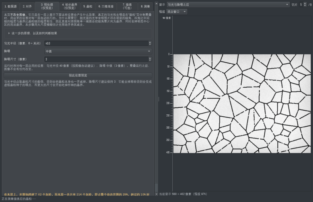
“预处理”页，图像显示的是匀光之后的结果。下方报告会说明灰度范围中有多少是光照造成的。

本步骤用大尺度模糊估计光照场并减去，并报告本层动态范围中有多大比例属于光照，便于您判断是否起了作用。

半径在两个方向上的风险并不对称。 取得过大只是少去掉一些暗角，而报告会让这一点显现出来；取得过小则低于晶粒尺度，会让每一层都不稳定：在一个已知含 36 个柱状晶粒的模型上，半径取 12 像素时每层数量依然正确，但层间一致性掉到 0.47，三维连接碎裂成 107 个晶粒、高度中位数仅 3 层，而正常应为 41 个、高度 8 层。建议值随图像尺寸缩放，并设有下限来防住这个危险方向。

5. 标签页 4 — 初步晶界

本页同样不改变任何东西 [2026-09-06b]：它只是在一层上预览下面的阈值设置会得到怎样的网络，让您在花时间跑整叠之前先判断有没有漏。运行时会用同样的设置对每一层自动计算这个网络。

标记深色网络。匀光之后通常 Otsu 就足够；手动灰度与局部自适应均值用于腐蚀深度变化快于匀光所能消除的情况。小于设定面积的暗点会被忽略，因为 4 个像素的斑点是脏物，否则会把一个晶粒切成两半。

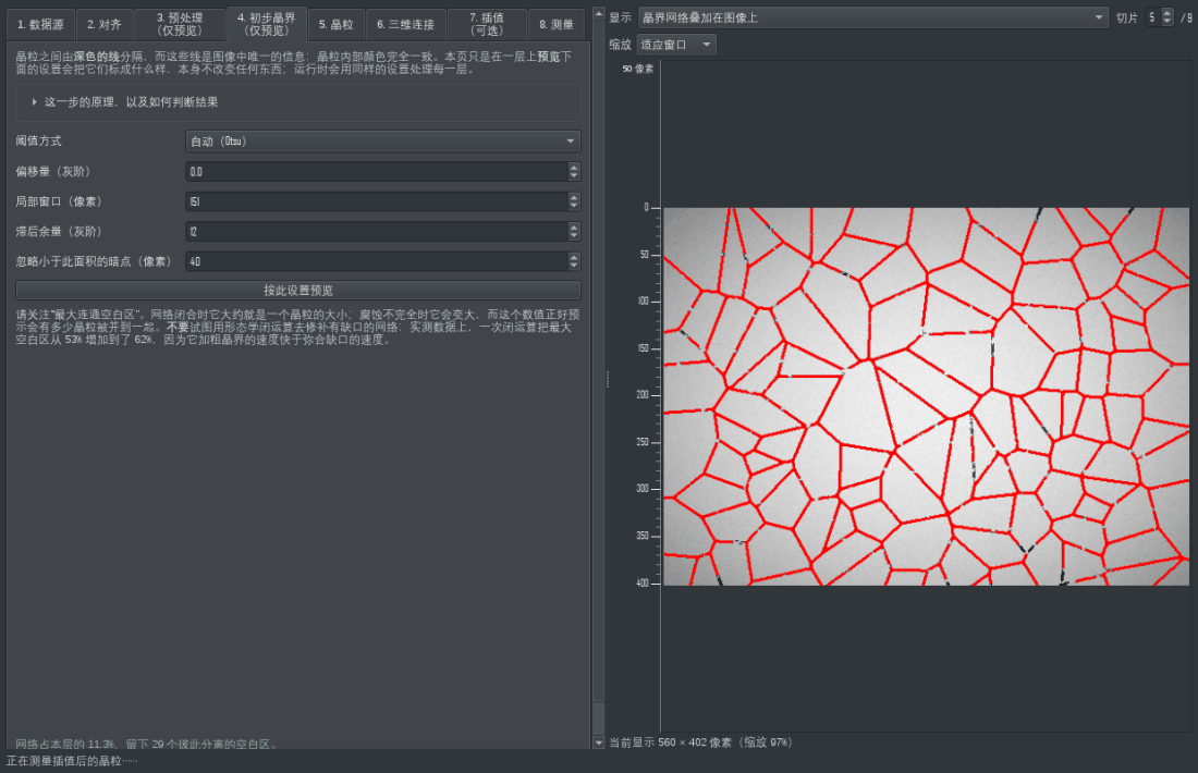
「初步晶界」页：提取到的暗色网络以红色叠加在图像上；报告给出“最大空白区域”，它预示会有多少晶粒被并到一起。

请关注“最大连通空白区”。 它是补集中最大连通区域占本层的比例，正好预示会有多少晶粒被并到一起。网络闭合时它大约是一个晶粒的大小。在参考数据上，匀光后是 38%，不匀光则是 53%。

不要用形态学闭运算去修补有漏的网络。 在真实数据上实测，一次闭运算把最大空白区从 53% 增加到了 62%——它加粗晶界的速度快于弥合缺口的速度。弥合缺口是下一步分水岭的职责。

这一页产出的东西不是插件最终发布的晶界。 它有好几个像素宽，而且在腐蚀不足的地方是断的；它唯一的作用，是充当下一步分水岭漫流的地形。您最终得到的晶界是在标签页 8 由完成后的晶粒导出的，只有一个像素宽，连通而且完整。

滞后阈值 [2026-09-06] 是第四种阈值方式，用于局部腐蚀较淡的样品。Otsu（加偏移量）决定沟槽确定存在的位置；比它再亮不超过“滞后余量”的像素也算作沟槽，但只有与某个确定的沟槽像素相连时才算。晶粒内部的噪声不与任何沟槽相连，所以不会被标出。在参考数据上实测：余量取 12 时，正常层的最大连通空白区减半，欠蚀刻层的从四分之三降到一半以下，而标出的像素中只有二十分之一远离 Otsu 网络；超过 18 就开始把内部噪声也标进去。Otsu 仍是默认：在整叠参考数据上，滞后网络得到 1,633 个晶粒而 Otsu 得到 1,439 个，没有真值能判断哪个更对。

6. 标签页 5 — 晶粒

两条路线。把整叠切片当作一个体积做一次三维分水岭（推荐，默认）：对齐后的整叠被当作一个体积，上下两层的暗色晶界墙会以“山脊”的形式出现在腐蚀不足那一层的距离图里，所以即使某一层丢了晶界，两个晶粒仍然分开；而且每个晶粒贯穿整叠只有一个种子，之后不需要任何连接。每层单独分割，再做三维连接是旧路线，保留下来以便在新样品上对比。

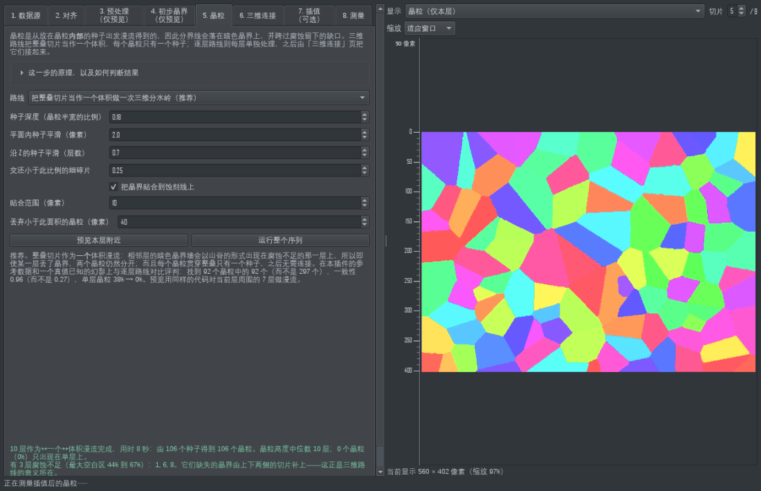
「晶粒」页的三维路线。种子深度以实测晶粒半宽的比例给出，同一个设置既适合粗晶也适合细晶；预览用与完整运行相同的代码对当前层周围的七层做漫流。

为什么用三维——实测。 在参考数据上，逐层路线把 20,439 个二维晶粒变成 1,905 个三维晶粒，其中 435 个只出现在单层上；同时四个腐蚀不足的切片把相邻晶粒粘在一起。四种重新设计在同一套评分框架上比较（一个真值已知、故意做坏两层的幻影，加上真实数据的一块裁切）：三维分水岭在幻影上找到 92 个晶粒中的 92 个（逐层路线为 297 个），在真实裁切上没有任何内部晶粒只出现在单层（逐层路线为 38%）。在整叠上它用时 7 分钟，得到 1,439 个晶粒，没有一个只在单层上，腐蚀不足的切片上有 527 个区域（好的切片上为 551 个）——那些层丢掉的晶粒回来了。

参数。 种子深度（晶粒半宽的比例）：调高则合并，调低则拆分。种子平滑分平面内与沿 Z（以层为单位；晶粒沿 Z 的轮廓更嘈杂，因为晶界墙在相邻截面之间会移动）。交还细碎片：晶界墙移动的地方，一个晶粒可能在下一层占走邻居截面的一条细带；在该层上小于晶粒主体这一比例的碎片会被交还。丢弃小于此面积的晶粒用于去掉斑点。

先预览。 三维预览需要已载入的整叠（它的种子来自相邻层），对当前层周围的七层做漫流。逐层路线的预览只需一层，不必载入。

把晶界贴合到蚀刻线上 [2026-09-06] 在三维路线中默认开启。三维洪泛只凭距离图决定每个体素属于哪个晶粒，所以它画出的分界线可能落在蚀刻沟槽旁边而不是沟槽上：在参考数据上实测，发布的晶界线像素中有 31% 落在比 Otsu 阈值更亮的灰度上，21% 离任何沟槽像素超过 4 像素。因此洪泛之后，每一层的分界线会被逐个晶粒地移到沟槽上，且只在“贴合范围”内移动：每个晶粒都保持自己的身份（比范围更薄的晶粒保留一个自己的种子），而在腐蚀没有留下沟槽的地方，线就留在洪泛放置它的位置。沟槽本身仍按中轴线分给两侧晶粒，和金相学家画晶界的方式一致。在整叠参考数据上实测，落在沟槽上的晶界线比例从 69% 升到 78%，晶粒仍是同样的 1,439 个，40 层的运行多花约 4 分钟。预览只贴合所显示的那一层。

7. 标签页 6 — 三维连接

一个晶粒是贯穿整个序列的单一对象。当相邻两层的两个二维晶粒重叠足够多时，它们属于同一个三维晶粒。

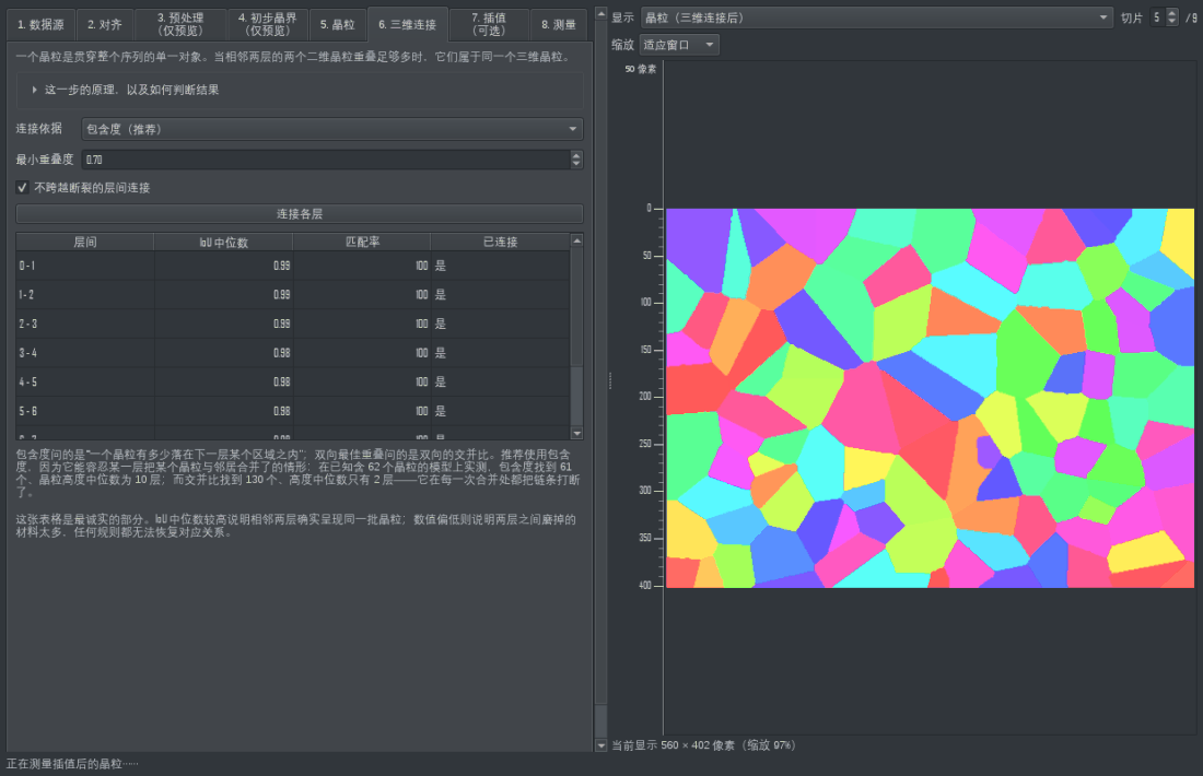
“三维连接”页：每一对相邻层一行，无法跟踪的层间会被明确报告出来，而不是靠猜测连接过去。

在三维路线上这一页无事可做：晶粒已经在整叠中携带同一个编号。表格仍会填上——显示三维结果相邻层之间的一致程度——按钮则不可用。它只是逐层路线的后半步。

默认使用包含度，理由是实测得出的。 包含度问的是“一个晶粒有多少落在下一层某个区域之内”；交并比问的是双向对称的重叠。当下一层的分割把某个晶粒与邻居合并了，交并比会骤降，尽管该晶粒明显仍在延续——在已知含 62 个晶粒的模型上，按交并比连接得到 130 个晶粒、高度中位数 2 层，而按包含度得到 61 个、高度中位数 10 层。

层间表格是本插件最诚实的部分。 它对每一对相邻层报告最佳 IoU 的中位数：数值高说明两层确实呈现同一批晶粒；数值低说明两层之间磨掉的材料太多，任何规则都无法恢复对应关系。这样的层间会被报告为断裂，并且默认不做跨层连接——在该处把晶粒切断，而不是靠猜测把它们连起来。

在参考数据上，39 个层间中有 33 个追踪良好（IoU 中位数 0.68），6 个断裂（0.27 至 0.49）。本流程的天花板是 0.98，由同一层加噪声重新分割测得。因此 0.7 左右是好结果，而不是勉强。

8. 标签页 7 — 插值（可选）

台阶问题。 连续切片在 Z 方向的间距远大于像素尺寸：参考序列的层间距为 0.5 um，而像素只有 0.0586 um，相差 8.5 倍。从一层到下一层，晶界的位置中位数移动 3.2 像素，十分之一的晶界移动 11 像素以上。因此由实测切片直接建成的三维 ROI 或网格，每个晶粒都像一叠边缘垂直的平板。数据本来就是这样，除非您运行本页，标签页 8 也正是按原样测量的——但它不好看，也不是晶粒真实的样子。

这一步被特意放在测量之前。 一旦按下对整个序列插值，“测量”页处理的就是这个体：表格、CSV 以及它发布的每一个对象都描述插值后的晶粒，对象名称中也会写明。跳过本页，或者按下丢弃它，测量切片被切出来时的原样，“测量”页就回到切片被切出来时的原样。无论选哪一种，分割本身都不会改变：插值只是在已经找到的晶粒之间补充层，它绝不会重新判定某个体素属于哪个晶粒。本页没有“发布”按钮——发布是“测量”页的职责，这样发布出去的永远就是测量过的那个对象。

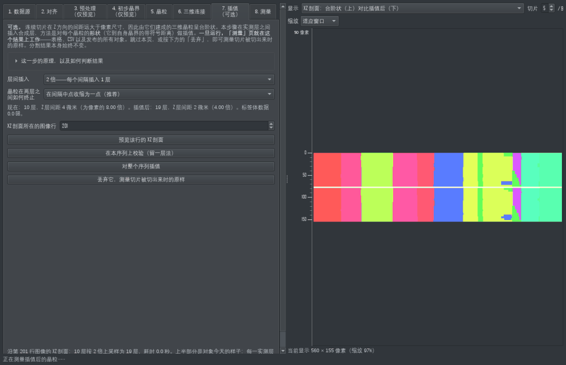
“插值”页：倍数下方给出插值前后的 Z 间距；XZ 预览的上半部分是对象今天的样子，下半部分是插值后的对象；下方的检验在您自己的序列上做“留一层”测试并报告结果。“对整个序列插值”把这个体交给“测量”页，“丢弃它，测量切片被切出来时的原样”则把实测切片交还回去。

本页做什么。 它在每一个层间隙里插入合成层：倍数 2 插 1 层，倍数 4 插 3 层，倍数 8 插 7 层，因此 40 层实测切片在 8 倍下变成 313 层。对每一个晶粒，取它在下一层和上一层上到自身晶界的带符号距离，按在间隙中的位置做线性混合，再把混合后距离最大的那个晶粒的标签赋给每个合成体素。正是最后这一步使结果成为一个划分——每个体素恰好属于一个晶粒，既不重叠也不留空——这也是它与“逐个晶粒单独插值”的根本区别。实测切片逐位精确地保留在原位；最后一层之外不凭空生成任何东西。只出现在一层、下一层已不存在的晶粒，以一个顶点位于间隙中点的圆锥收尾：切片并没有说出这个晶粒究竟在哪里结束，本页就把终点放在正中间并如实说明，而不是假装知道。

插值前后的 Z 间距。 本页把您序列的层间距与面内像素并列打印，并给出插值后对象将携带的间距：参考序列在 8 倍下 Z 间距由 0.5 um 变为 0.0625 um，即体素从 8.5 : 1 变为 1.07 : 1，接近立方。请根据这两个数字选倍数——目标是让体素的高与宽大致相当，而不是选最大的那个倍数。

1. 选择倍数（2、4 或 8），在运行任何东西之前先读一下它下方的内存与时间估计。

2. 把行滑块移到视场中的某一行，阅读 XZ 预览：上半部分是对象今天的原样——每个实测层一块平板；下半部分是同一行插值之后的样子。两半都是精确计算的，不是示意图。

3. 点击 在本序列上校验（留一层法），在您自己的序列上运行这个测试；阅读它返回的两个数字（见下文）。

4. 点击 对整个序列插值。完整的插值体在工作线程中构建，面板保持可用。

5. 切到 测量 页。它的摘要现在第一行就写明这是插值体、倍数是多少、Z 间距是多少；它发布的每个对象名称里也都带有这个倍数。

6. 改变主意了？点击 丢弃它，测量切片被切出来时的原样。“测量”页会回到实测切片并明确说明，其它什么也不会丢失。

内置检验，以及如何读它

从未切出的那一层无法用来验证，于是本页用切出来的层验证：去掉一层实测切片，用它的两个邻层把它重建出来，再与真实的那一层比较。重建层用两种方式打分——标签正确的像素比例，以及重建晶界与真实晶界之间距离的中位数（像素）。两个数字对“台阶式直接复制”和“插值”各报一份，并排给出，所以您看到的是在您自己的数据上的改善，而不是我们的。这个测试的间隙是两个层间距，是本页实际填补间隙的两倍，因此数字偏保守。参考序列上，检验报告台阶式为 3.2 像素、插值为 1.2 像素（像素正确率 0.884 对 0.949）。

为什么没有选更花哨的方法。 同一个测试在整个参考序列上对每一种被提议的更强方法都跑过一遍，晶界误差中位数如下：

• 最近邻复制（现状的台阶）：3.1 像素
• 逐晶粒带符号距离混合——本页所做的：1.1 像素
• 先用 Demons 弹性配准把两个邻层各向对方变形一半、再做同样的混合：1.1 像素，完全相同——尽管配准确实把晶界移动了实测的每层位移量
• 先把每个晶粒按各自质心对齐、再做同样的混合：1.5 像素，更差
• 穿过四层的三次曲线代替穿过两层的直线：1.4 像素，更差

混合仍然做错的部分中，94% 位于两个邻层上都存在的晶粒内部——那是晶界在间隙内部的形状，两张切片根本不携带这一信息，任何方法都无法从中恢复。所以两层线性混合就是本页的方法；任何声称更好的方法，都必须在这个测试上做到优于 1.1 像素。

内存与时间

8 倍下，参考序列（40 × 1945 × 2386）变为 313 层、2.9 GB 的标签体，构建约两分钟（实测 80–124 s，峰值工作集 3.6 GB）。本页会在运行前打印您的序列在所选倍数下的大小。内存不足时请选 4 倍或 2 倍：对象小 4 到 8 倍，而台阶已经大为减少。

在插值体上测量时，哪些数字会变、哪些不会

• 晶粒体积几乎不变，甚至可以说更合理。 实测表格本来就把每个体素乘以完整的层间距（参考序列是 0.5 um），也就是说它已经把每一层沿整个间隙拉伸了一遍，并在切片处留下一堵垂直的墙。插值并不增加体积，它只是把这种拉伸换成一个在间隙中平滑移动的晶界。样品的总体积几乎不变：序列的最顶层与最底层各让出半个层间距（那里没有第二张切片可供插值），因此插值后的总体积为实测总体积的 ((Z - 1) + 1/倍数) / Z——40 层序列在 8 倍下为 97.8%，10 层序列为 91.3%。相邻两个晶粒之间此消彼长的，只是两种处理方式对间隙的理解不同的那一部分。
• “跨越层数”这一列数的是插值层。 跨越 5 个实测切片的晶粒，若两端都在序列内部，在 8 倍下读作 39 层；若有一端正是序列的顶面或底面，读作 36 层；两端都在面上时读作 33 层。请改为引用以微米计的高度——面板会在摘要的第一行把它打印出来：倍数、层数、Z 间距，以及跨度中位数（同时给出层数和高度）。这个高度与实测值接近，但并不完全相同：内部晶粒会少掉一个插值层（层间距 ÷ 倍数，参考序列在 8 倍下为 0.0625 um）；而以序列表面收尾的晶粒，在那一端会少掉半个层间距——因为实测表格把它的端层沿完整层间距拉伸，而插值体就停在那张切片本身。引用时请说明数字取自哪个对象。
• 一个像素宽的晶界 ROI 是逐插值层绘制的，因此它的体素数量大致按倍数增加，而每个体素又薄了同样的倍数。晶界规模只能在用同样方式构建的对象之间比较，绝不要拿实测网络与插值网络相比。
• 合成层里没有任何新信息。 它只是与上下两张切片都相容的最平滑形状，因此一条在间隙内部其实是折线的晶界，会被画成光滑的。残差恰恰就在这里：混合仍然做错的部分中，94% 位于两个邻层上都存在的晶粒内部。插值并不能让您引用比切片间距所能支撑的更精细的特征。

⚠ 任何数字都要说明它来自哪个对象。 本插件的两个结果，只有在同一类对象上测得时才可比。正因如此，CSV 里有 source 列（measured_sections 或 interpolated_x8）和 slice_thickness 列，发布出去的名称里带有 (interpolated x8)，摘要的第一行也写明对象。插值是对切片间隙的一种解释——一种站得住脚的解释，上表也说明了它能被信任到什么程度——但它不是额外的数据。

如何对比有无插值： 测量并发布两次。先运行插值、在“测量”页发布，再按丢弃它，测量切片被切出来时的原样、重新发布一次——两个对象位于同一网格、同一原点，其中一个名字里带着倍数。在 Dragonfly 中把一个 2D 视图切到 XZ 或 YZ，在两者之间切换；或者各建一个网格：实测对象的平板对比插值对象的平滑侧面。

9. 标签页 8 — 测量与发布

摘要的第一行会说明这些数字描述的是哪个对象。 如果您运行过标签页 7，本页测量并发布的就是插值体，并写明它的倍数与 Z 间距；如果您没有运行、或者在那里按了“丢弃”，本页测量的就是切片被切出来时的原样，也不会多说什么。除此之外，本页的其它行为不因这个选择而改变。

每个晶粒：体素数、体积、等效直径，以及跨越了多少层。最后这一列值得单独看：只存在于一层的三维晶粒说明它从未与任何东西连接，而满表都是这种晶粒意味着连接失败，而不是晶粒本身扁平。在插值体上，这一列数的是插值层——跨越 5 个实测切片的晶粒在 8 倍下约读作 39 层，若有一端正是序列的表面则更少——因此请引用摘要中一并给出的、以微米计的高度，并说明它取自哪个对象（其中的算术见标签页 7）。

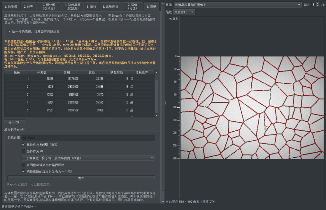
“测量”页，图中已经运行过插值：第一行就是插值提示，写明倍数与 Z 间距，“跨越层数”一列数的是插值层。其下是每个晶粒的体积与等效直径、D10/D50/D90 分布，以及有多少晶粒接触到体数据的表面——那些晶粒的尺寸只是下限。

与体数据表面相接的晶粒是被截断的，其测得尺寸只是下限。 层数较少时几乎每个晶粒都会碰到顶面或底面——在一次 10 层的测试中占 85%——因此“仅内部晶粒”的平均值会与整体值并列给出，您应明确说明自己引用的是哪一个。

发布会把晶粒作为 MultiROI 加入（每个晶粒一个标签，并以其尺寸命名），可选把晶界网络作为 ROI 加入。几何信息从源通道复制，因此结果精确落在它所来自的图像上。另有两个默认勾选的选项：“同时发布对齐后的图像”把对齐并裁剪后的灰度图像与晶粒、晶界一起发布（仅当已对齐且未插值）；“不与表面接触的晶粒作为单独的 MultiROI”再发布一个只含尺寸完整晶粒的 MultiROI，标签重新连续编号，名称中带有表格里的晶粒编号。

当插值结果有效时，发布有四处不同。 每个对象名称都会加上 (interpolated x8)。写入对象的 Z 间距是切片步距除以倍数——8 倍下是 0.0625 um 而不是 0.5 um——因此在 Dragonfly 中量出的距离是对的（这一覆盖已在运行中的 Dragonfly 里验证过：在 0.5 um 的源通道上以 4 倍发布的 MultiROI，读回来是 Z = 0.125 um）。对齐后的灰度图像不会随之发布，因为它只有实测的 40 层，而标签有 313 层，两者不在同一网格上。而且在对齐过的序列上，如果 Dragonfly 不接受移动后的原点，发布会带着原因失败，而不是退回源坐标系：那种退回要撤销每层的整像素平移，而合成层并没有属于自己的平移可撤销。

CSV 中包含每一个晶粒，另外还有两列记录“测的是什么”：slice_thickness，即该行所来自对象的 Z 间距；以及 source，取值为 measured_sections 或 interpolated_x8。默认文件名也会因此加上 _interpolated_x8。把数字粘进报告时，请一并保留这两列。

选取部分切片范围时拒绝发布，并给出原因：新对象会继承源通道的原点，在 Z 方向落错位置。请载入完整范围，或改为导出 CSV。

晶界 ROI：一个像素宽，连通、闭合

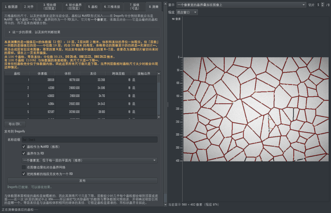
最终发布的晶界，叠加在图像上：只有一个像素宽；有腐蚀线的地方它沿着线走，没有的地方它径直穿过缺口，因此不会有两个晶粒仍然连在一起。

最终发布的晶界不是标签页 4 的阈值结果，而是由完成后的晶粒导出的：每一对相邻晶粒之间都画出一条一个像素宽的线，无论腐蚀是否在那里显出过线条。因此两个晶粒总是被分开的，网络不会断，您可以沿着它走、量它的长度，或者把它当作掩膜使用。

线条按 8 邻接连通，它围出的晶粒按 4 邻接——这是标准的一对，也是线条走对角线时不会漏的原因。发布之后，报告会给出网络的规模、它由多少个连通片段组成，以及有多少像素（如果有的话）没能细化到一个像素。最后这个数字应当是零；如果不是，那是四个晶粒在一个 2×2 内交汇的位置，任何一个像素宽的线条都无法表达——这不是可以调参解决的问题。

• 一个像素宽，位于每一层的平面内是推荐方式，也是默认值。在参考数据上它约占体积的 3%。
• 三维界面壳层是更早的理解方式：所有与不同标签面相邻的体素，两个体素厚，在参考数据上占体积的 38%。它回答的是另一个问题；在层数很少的序列上，它几乎没有意义。
• 在图像边缘处闭合晶界网络会额外把边框画上，使被视场边缘切断的晶粒同样闭合。这些像素并不是真正的晶界——如果您要测量晶界长度，请不要勾选。

线条像素必须从它所分开的两个晶粒中的某一个身上取走，因为在像素网格上没有别的地方可以画它。所以晶界 ROI 与晶粒 MultiROI 是重叠的，晶粒仍保持表格中的尺寸；如果您需要两者互不重叠，请在 Dragonfly 里用MultiROI 减去这个 ROI。发布之前想先看看这张网络，请把图像选择器切到「晶界（一个像素宽）」——那正是「发布」将要交出去的那个数组。

有支撑的线与推断的线 [2026-09-06] 一个线像素若在本层 2 像素以内有蚀刻沟槽像素，就算有支撑；其余的线是推断出来的——它记录的是三维洪泛判定两个晶粒相接的位置，而本层图像上没有对应的沟槽（通常是欠蚀刻层）。完整的一像素网络照常发布；勾选“把纯推断的线段另发布为一个 ROI”（默认勾选）后，推断部分会作为第二个 ROI 发布，名称以 inferred 结尾，报告会给出有支撑的比例，预览模式“晶界叠加在图像上：有蚀刻支撑（绿）、纯推断（品红）”会把两者画在图上。插值体积不提供此项：其合成层背后没有图像。

10. 如何判断您的序列究竟能不能做三维重建

这是在相信任何三维数值之前必须先解决的问题，而插件已在标签页 5 的表格中替您回答了。

• 如果多数层间的 IoU 中位数在 0.6 以上，说明层间距足够小，晶粒可以被追踪。
• 如果多数层间数值都低、且多数晶粒只跨一层，说明每次抛光磨掉的材料约相当于一个晶粒的厚度。这不是算法能弥补的，必须用更小的步距重新制样切片。经验法则：让您关心的最小晶粒至少被切出五层。
• 若一个总体良好的序列中只有个别断裂，那只是把序列分成了若干段。两次断裂之间的每一段都是有效的三维体，请分段测量，而不要跨越断裂给出一个整体数值。

11. 本插件不做的事

• 不测量取向，因此这里的任何结果都无法转成取向差、孪晶判定或极图。腐蚀金相照片本身不含取向信息。
• 它不做完整的配准。 标签页 2 只修正每层一次的整像素平移，除此之外什么也不做：不做旋转、不做缩放、不做亚像素平移、不做弹性变形。需要这些的话，请先用 Dragonfly 自带的 Slice Registration，再回到本插件。
• 不做亚像素晶界定位。 一条晶界就是一个体素面。
• 不区分物相、不识别夹杂物；腐蚀留下的暗斑仅按面积被当作晶界或脏点处理。
• 不假定晶粒是紧凑的。 插件报告的等效直径隐含了这个假定，因此对柱状组织请改看体积与跨越层数。

9. 网格（可选）。 把晶粒转换成彼此仍然紧密接触的三角网格。这里为整个多晶体构建一个网格，顶点是共享的：两个晶粒之间的面只存在一次、同时属于两者，平滑时移动的是那一个面，两个晶粒随之一起移动。逐个晶粒分别构建再分别平滑做不到这一点——各表面会到处相差不到一个体素地彼此错开；对晶界 ROI 做网格化同样不行，那条一个体素宽的带子经 marching cubes 之后是一个由相隔一个体素的两张面构成的壳。目标体素尺寸默认取原图自身的 Z 层间距，因为相邻两个截面之间的形状是推断出来的、而不是测得的：在参考数据上，按像素尺寸做网格得到 7600 万个三角面，其中 87% 是相邻层之间的水平壁，也就是台阶本身；而按 Z 层间距只有 190 万个。平滑默认用 Taubin（能保持体积；普通 Laplacian 会让同一批晶粒缩小约 2.5%），每个顶点都被限制在自己那半个体素的小格内，三个或四个晶粒相交处的顶点则被限制或完全固定，从而保住三叉棱线和角点。报告会说明每个晶粒是否封闭、法线是否朝外，以及其体积与来源体素计数的对比；旁边的图像把网格被当前层截出的轮廓画在原图之上。可以把多晶体作为一个 Mesh 发布，也可以按上限逐个发布晶粒，或者把每个晶粒导出为二进制 STL——要导出成千上万个晶粒，应该走这条路。

Part II English Manual

Contents

1. Introduction

2. Tab 1 - Source

3. Tab 2 - Align (optional)

4. Tab 3 - Preprocess

5. Tab 4 - Preliminary Boundaries

6. Tab 5 - Grains

7. Tab 6 - Link 3D

8. Tab 7 - Interpolation (optional)

9. Tab 8 - Measure and publish

10. How to tell whether your stack can be reconstructed at all

11. What this plugin does not do

1. Introduction

An etched metallographic micrograph shows grain boundaries as dark lines on a matrix where every grain interior looks the same. All of the information is in the boundary network, and this plugin segments that network, slice by slice, then links the result into three-dimensional grains.

The eight tabs are the workflow itself. Each opens only once the step before it has produced something, so the panel cannot be used out of order by accident. The seventh, Interpolation, is optional and it sits before the measurement on purpose: if you run it, the eighth tab measures and publishes the interpolated volume; if you skip it, or discard its result, the eighth tab measures the sections exactly as they were cut. Nothing is created in your session until you press a Publish button - Tab 2's optional aligned image, or Tab 8's results. A ninth, Meshing, is optional and comes last: it turns the measured grains into triangle meshes that still touch.

Why this is not the EBSD plugin, and not a colour segmentation. In an EBSD map the grain identity is the orientation measured at each pixel. Here there is no orientation at all, and the interiors carry no distinguishing colour: measured on a reference stack, the CIE76 colour difference between the interiors of different grains is 7.2 - noise - while matrix-versus-boundary is 49.5. A method that clusters or region-grows on interior colour therefore cannot separate these grains at all. If you have orientation data, use 3D EBSD; if you have a colour picture of an IPF map, Color Image Processing says plainly that it decodes no orientation.

In the image area: scroll the WHEEL to step through the slices, drag with the MIDDLE button to zoom (the point under the cursor stays put), and hold the LEFT and RIGHT buttons together and drag to pan. The ruler down the left edge is graduated in image pixels and follows the zoom, and the line under the image says how much of the image is on screen — every parameter in this plugin is expressed in pixels, so that is the number you need when choosing one. Beside the slice number the panel prints the number Dragonfly's own view gives the same slice (Dragonfly may count from the other end), and the preview is mirrored whenever Dragonfly's current 2D view draws the image mirrored, so the two show the same picture the same way up. Show in Dragonfly moves Dragonfly's current 2D view to the slice you are looking at here. Both are read from the live view each time the preview redraws; if that view is not an XY slice view of the image, the panel says so and the button is disabled.

Execute All Steps with Current Settings on the Source tab runs the whole workflow unattended - load, align, commit the preprocessing and boundary settings, segment the grains, link, publish - each step with whatever its own tab shows at the moment you press it, so a run that takes the best part of an hour can be started and left. Interpolation and meshing are OFF by default because they are the expensive ones, and alignment is ON because the Align tab's own auto-apply is; each is a tick box beside the button and a skipped step is written into the log. Every tab stays open at all times so that all of those parameters can be read and changed BEFORE the run: a step whose input does not exist yet refuses when you press ITS button and says which step is missing.

2. Tab 1 - Source

Pick the image already imported into Dragonfly. The voxel size comes from the channel, so calibrate the image in Dragonfly once and every length in this plugin is in micrometres. If Dragonfly reports no voxel size, the panel says so and every length is labelled in voxels instead of quietly pretending.

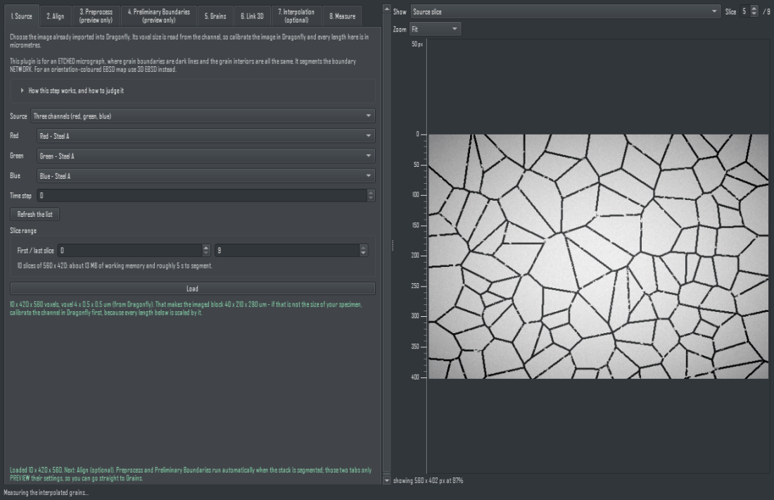
The Source tab. The channels, the slice range, and the memory and time the run will cost — printed before you commit to it.

• One channel for a grey image, or for one band of a colour image.
• Three channels for a colour image Dragonfly split into Red / Green / Blue. They are paired by name: the first title whose leading word is 'Red', then the Green and Blue whose names match that same image. Pairing by position would join 'Green - Sample 2' to 'Red - Sample 1' whenever two colour images are open.

The three bands are combined with the standard luma weights. The slice range lets you work on part of the stack while tuning; the memory and the time it will cost are printed before you commit, because the reference stack is 207 million voxels.

3. Tab 2 - Align (optional)

⚠ Dragonfly already has a full Slice Registration tool, and it is the better one. Right-click your dataset in the Data Properties and Settings panel and choose Slice Registration: it offers enhanced correlation coefficient, feature-based, mutual information, SSD, optical flow and template matching, rotation as well as translation, a drift compensator, manual editing slice by slice, and transformation templates you can save and reuse. Use it whenever the slices are rotated, distorted or badly out of register, or whenever the alignment itself is part of your result.

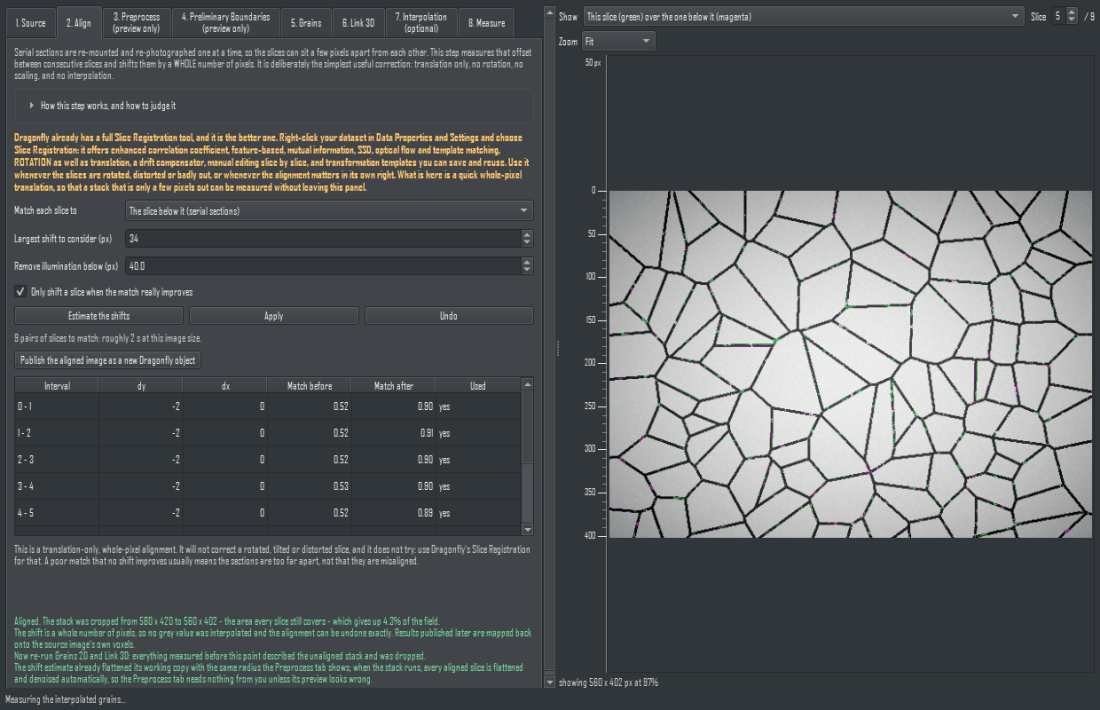
The Align tab. Dragonfly's own Slice Registration is named at the top; below it, the measured shift for every pair of slices with the match before and after it.

This tab is deliberately the smallest useful correction, so that a stack which is only a few pixels out can be measured without leaving the panel: one whole-pixel translation per slice. No rotation, no scaling, no sub-pixel shift, no interpolation. It is optional - skip it when the slices already sit on top of each other.

1. Set the view above the image to This slice (green) over the one below it (magenta) and walk the slider through the stack. Where two slices agree the colours cancel to grey; a misalignment shows as a coloured fringe as wide as the error.

2. Press Estimate the shifts. Each pair of neighbouring slices is matched by cross-correlation and the table fills in: the shift found, and how well the two slices matched before and after it. Nothing has moved yet.

3. Read the table. A shift is only worth taking when match after is clearly above match before; the column marked Used says whether it was.

4. Press Apply. The slices are shifted and the stack is cropped to the rectangle every slice still covers - the panel reports how much of the field that costs.

5. Undo puts the whole field back exactly, at any time.

6. Optional: Publish the aligned image as a new Dragonfly object sends the aligned slices into your session as a new image channel. The rest of this plugin does not need it — it is for using the aligned stack with Dragonfly's own tools, or for saving it. It is published at the SOURCE image's own size and position so it lines up with the original; the strip each slice was shifted in from outside the frame is left at zero, and the panel tells you the rectangle that holds real data on every slice. Crop it in Dragonfly if you want only that rectangle — Dragonfly's crop moves the origin with it, which is why this plugin does not hand you a pre-cropped object.

7. Apply the shift as soon as it is estimated is ticked by default, so Estimate also applies the shift in the same step and Undo still takes it back exactly; untick it to read the table first and press Apply yourself. The tick is remembered between sessions.

Why whole pixels. Every later step thresholds the thin dark boundary lines, which are the only information in an etched micrograph. A sub-pixel shift or a rotation has to resample the image, and resampling blurs exactly those lines. A whole-pixel shift moves the data and changes no value; it is also exactly invertible, which is what lets grains measured on the aligned stack still be published onto the original image's own voxels.

Align before you judge the specimen. An interval that still matches poorly after shifting is genuinely a break: too much material was polished away between those two slices, and no registration recovers it. But an interval that is merely TRANSLATED looks identical to a break, because its grains do not overlap - measured on the reference stack, six intervals that Tab 6 reported as breaks all tracked normally once the slices were aligned, one of them going from 0.00 to 0.56 after a 61 px shift. Run this tab first, then read Tab 6's table.

4. Tab 3 - Preprocess

This tab changes nothing in the image [2026-09-06b]. It previews, on one slice, what the flatten radius and the denoise setting will do; the flattening and denoising themselves are performed automatically, slice by slice, when the stack is segmented on the Grains tab, with exactly the settings shown here (the radius is suggested from the image size when the stack loads). You can go straight from Source, or from Align, to Grains; come back here only when the preview or the boundary network looks wrong. The alignment already flattens its own working copy with the same radius before it estimates the shifts, so aligning first does not require anything on this tab either. The tab title says preview only for this reason.

An optical micrograph of a polished section vignettes. Measured on the reference data, the illumination field spans 35% of the grey range - about as much as the boundaries are darker than the grains - so a single threshold on the raw image keeps the dark corners as boundary and loses the faint boundaries in the bright middle.

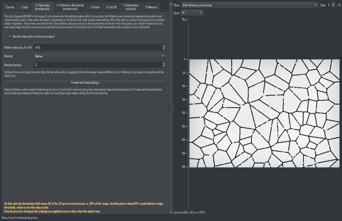
The Preprocess tab, with the image shown after flattening. The report states how much of the grey range was illumination.

The field is estimated with a wide blur and subtracted, and the panel reports what fraction of the slice's range was illumination so you can see whether it worked.

The radius matters in one direction more than the other. Too large removes less of the vignette, which the report makes visible. Too small is below the grain scale and destabilises every slice: on a phantom whose 36 columnar grains were known, a radius of 12 px still gave the right per-slice count but the slice-to-slice agreement fell to 0.47 and the 3-D link fragmented into 107 grains of median height 3 instead of 41 of height 8. The suggested value scales with the image and is floored to protect that direction.

5. Tab 4 - Preliminary Boundaries

This tab, too, changes nothing [2026-09-06b]: it previews the network that the threshold settings below produce on one slice, so you can judge the leak before paying for the whole stack. The run computes the same network for every slice automatically with these settings.

Mark the dark network. Otsu is usually enough after flattening; a manual level and an adaptive local mean are there for a slice whose etch depth varies faster than the flattening removes. Dark specks below a size are ignored, because a four-pixel blob is dirt and would otherwise cut a grain in two.

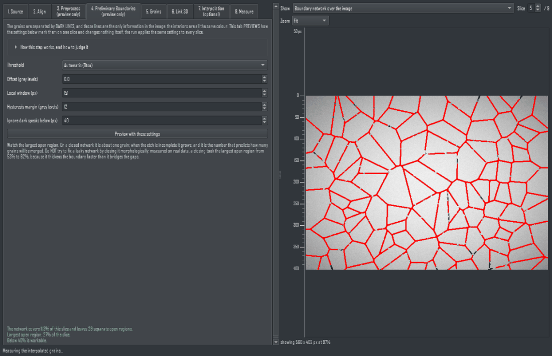
The Preliminary Boundaries tab. The dark network is drawn over the image in red, and the report gives the leak — the largest open region, which predicts how many grains will merge.

Watch the largest open region. That is the fraction of the slice taken by the biggest connected region of the complement, and it is the number that predicts how many grains will be merged. On a closed network it is about one grain. On the reference data it was 38% after flattening, and 53% without.

Do not try to fix a leaky network with a morphological closing. Measured on the real data, a closing took the largest open region from 53% to 62% - it thickens the boundary faster than it bridges the gaps. Closing the gaps is the watershed's job, in the next step.

What this tab produces is NOT the boundary the plugin publishes. It is several pixels wide and it is broken wherever the etch was weak; its one job is to be the landscape the watershed floods in the next step. The boundary you get at the end is derived from the finished grains on Tab 8, and it is one pixel wide, connected and complete.

Hysteresis [2026-09-06] is a fourth threshold for a specimen whose etch is faint in places. Otsu (plus the offset) decides where a groove certainly is; a pixel up to the hysteresis margin brighter than that still counts as groove, but only where it is connected to a certain groove pixel. Interior noise is not connected to anything, so it is not marked. Measured on the reference stack, a margin of 12 halves the largest open region on good slices and takes it from three quarters to under half on under-etched ones, while only one marked pixel in twenty lies away from the Otsu network; above 18 it starts marking interior noise. Otsu remains the default: on the full reference stack the hysteresis network gave 1,633 grains against 1,439, and there is no ground truth to say which is right.

6. Tab 5 - Grains

Two routes. One watershed over the whole stack, in 3-D (recommended, the default): the aligned stack is treated as one volume, the dark walls of the slices above and below stand on an under-etched slice as ridges in the distance map, so two grains keep their boundary where one slice lost it, and every grain gets ONE seed through the stack, so nothing has to be linked afterwards. Each slice on its own, then link is the older route, kept so the two can be compared on a new specimen.

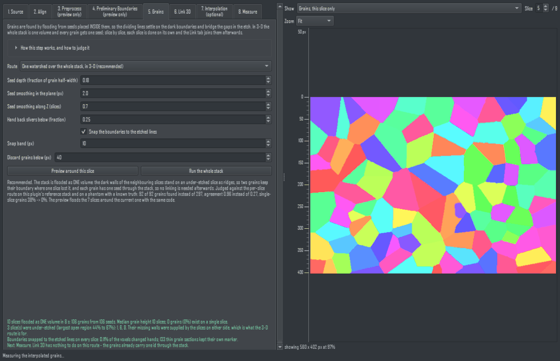
The Grains tab on the 3-D route. The seed depth is a fraction of the measured grain half-width, so one setting fits coarse and fine grains; the preview floods the seven slices around the current one with the same code as the full run.

Why 3-D, measured. On the reference stack the per-slice route turned 20,439 2-D grains into 1,905 3-D grains of which 435 existed on a single slice, while four under-etched slices glued neighbouring grains together. Four redesigns were scored on one harness (a phantom with a known truth and two deliberately under-etched slices, plus a crop of the real stack): the 3-D watershed found 92 of 92 phantom grains where the per-slice route found 297, and left no interior grain of the real crop on a single slice where the per-slice route left 38%. On the full stack it took 7 minutes, found 1,439 grains, none on a single slice, and the under-etched slices carry 527 regions against 551 on good slices - the grains those slices had lost are back.

The knobs. Seed depth (a fraction of the grain half-width): raise to merge, lower to split. Seed smoothing in the plane and along Z (in slices; a grain's profile along Z is noisier because the wall moves between sections). Hand back slivers: where a wall moved between sections a grain can claim a thin strip of its neighbour's cross-section on the next slice; pieces below this fraction of the grain's main piece on that slice are returned. Discard grains below removes specks.

Preview first. The 3-D preview needs the loaded stack (its seeds come from the neighbouring slices) and floods a 7-slice window around the current slice. On the per-slice route the preview works on one slice without loading.

Snap the boundaries to the etched lines [2026-09-06] is on by default for the 3-D route. The 3-D flood decides WHICH grain each voxel belongs to from the distance map alone, so its dividing lines can sit beside the etched groove instead of on it: measured on the reference stack, 31% of the published line pixels lay on grey brighter than the Otsu level and 21% were more than 4 px from any groove pixel. After the flood, every slice's lines are therefore moved onto the groove, grain by grain and only within the snap band: every grain keeps its identity (a grain thinner than the band keeps one marker of its own), and where the etch left no groove the line stays where the flood put it. The groove itself is still split down its middle between the two grains, as a metallographer draws the boundary. Measured on the whole reference stack the share of the line lying on the groove rose from 69% to 78% with the same 1,439 grains, at a cost of about 4 minutes on a 40-slice run. The preview snaps only the slice it shows.

7. Tab 6 - Link 3D

A grain is one object through the stack. Two 2-D grains belong to the same 3-D grain when they overlap enough between consecutive slices.

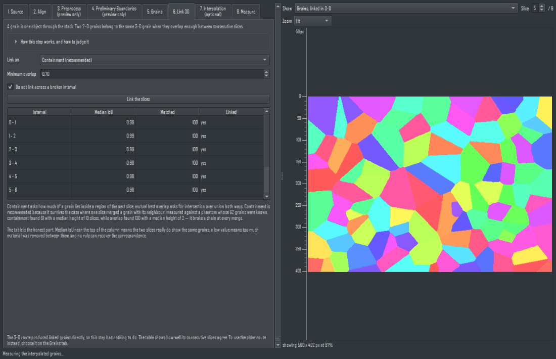
The Link 3D tab. One row per pair of neighbouring slices, so an interval that cannot be tracked is reported rather than linked on a guess.

On the 3-D route this tab has nothing to do: the grains already carry one id through the stack. Its table is still filled - with the slice-to-slice agreement of the 3-D result - and its button stands down. It is the second half of the per-slice route only.

Containment is the default, and the reason is measured. Containment asks how much of a grain lies inside a region of the next slice; intersection-over-union asks for the symmetric overlap. When the next slice's segmentation merges a grain with its neighbour, the IoU collapses even though the grain plainly continues - and against a phantom whose 62 grains were known, linking on IoU produced 130 grains with a median height of 2 slices while containment produced 61 with a median height of 10.

The interval table is the honest part of this plugin. For each pair of consecutive slices it reports the median best IoU: high means the two slices really do show the same grains, low means too much material was removed between them and no rule can recover the correspondence. Such an interval is reported as a break and, by default, not linked across - the grains are cut there instead of being joined on a guess.

On the reference stack, 33 of 39 intervals tracked well (median IoU 0.68) and 6 broke (0.27 to 0.49). The ceiling for this pipeline is 0.98, measured by re-segmenting one slice under noise. So a value near 0.7 is good, not mediocre.

8. Tab 7 - Interpolation (optional)

The stair-step problem. Serial sections are far apart in Z compared with the pixel: on the reference stack the step is 0.5 um against a 0.0586 um pixel, a factor of 8.5. Between one slice and the next a grain boundary moves by a median of 3.2 px, and one boundary in ten moves 11 px or more. A 3-D ROI or a mesh built from the measured slices therefore shows every grain as a stack of flat plates with vertical sides. That is what the data actually says, and Tab 8 measures it as it is unless you run this step - but it is hard to look at, and it is not what the grain looks like.

This step comes before the measurement on purpose. Once you press Interpolate the whole stack, the Measure tab works on THIS volume: the table, the CSV and every object it publishes describe the interpolated grains, and their titles say so. Skip this tab, or press Discard it and measure the sections as they were cut, and the Measure tab goes back to the sections exactly as they were cut. Either way the segmentation itself never changes: interpolation adds slices between grains that were already found, it never re-decides which voxel belongs to which grain. There is no Publish button here - publishing is the Measure tab's job, so that what is published is always what was measured.

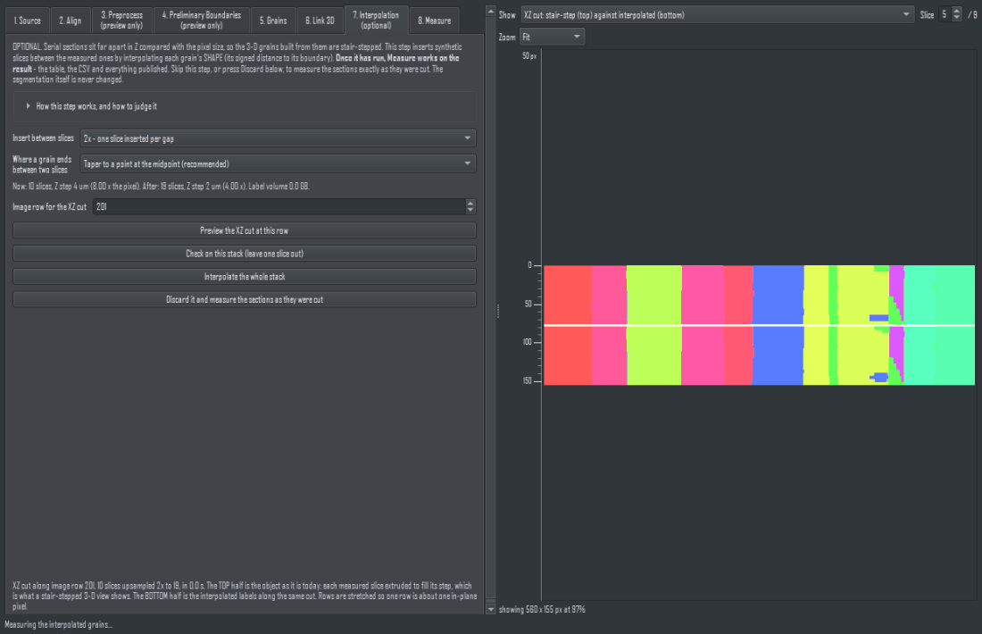
The Interpolation tab. The Z spacing before and after is printed below the factor; the XZ preview shows the object as it is today in the top half and the interpolated object in the bottom half; the check below reports the built-in leave-one-slice-out test on your own stack. Interpolate the whole stack hands the volume to the Measure tab; Discard it and measure the sections as they were cut hands the measured sections back.

What the tab does. It inserts synthetic slices into every gap: 1 at factor 2, 3 at factor 4, 7 at factor 8, so 40 measured slices become 313 at 8x. For each grain it takes the signed distance to that grain's boundary on the slice below and on the slice above, blends the two linearly by position in the gap, and gives every synthetic voxel the label whose blended distance is largest. Because of that last step the result is a partition - every voxel belongs to exactly one grain, nothing overlaps and nothing is left empty - which is what separates it from interpolating each grain on its own. The measured slices are kept bit-exactly where they were; nothing is invented beyond the last one. A grain that is present on one slice and absent on the next ends in a cone whose apex is at the midpoint of the gap: the section does not say where the grain really ended, so the tab puts the end half-way and says so, rather than pretending to know.

The Z spacing, before and after. The tab prints the slice spacing of your stack next to the in-plane pixel, and the spacing the interpolated object will carry: at factor 8 the reference stack goes from 0.5 um to 0.0625 um in Z, i.e. from 8.5 : 1 voxels to 1.07 : 1, nearly cubic. Pick the factor from these two numbers - the aim is voxels that are roughly as tall as they are wide, not the largest factor offered.

1. Choose the factor (2, 4 or 8) and read the memory and time estimate under it before anything runs.

2. Move the row slider to a row across the field and read the XZ preview: the top half is the object exactly as it is today - flat plates, one per measured slice - and the bottom half is the same row after interpolation. Both halves are computed exactly, not sketched.

3. Press Check on this stack (leave one slice out) to run that test on your own stack; read the two numbers it returns (below).

4. Press Interpolate the whole stack. The full interpolated volume is built on a worker thread; the panel stays usable.

5. Go to the Measure tab. Its summary now begins by naming the interpolated volume, its factor and its Z step, and everything it publishes carries that factor in its title.

6. Changed your mind? Press Discard it and measure the sections as they were cut. The Measure tab returns to the measured sections and says so; nothing else is lost.

The built-in check, and how to read it

Nothing here can be verified against a slice that was never cut, so the tab verifies against slices that were: it removes one measured slice, rebuilds it from its two neighbours, and compares. The rebuilt slice is scored two ways - the fraction of pixels carrying the right grain, and the median distance in pixels between the rebuilt boundary and the real one. Both are reported for the plain stair-step copy and for the interpolation, side by side, so you see the improvement on your data rather than on ours. The gap in this test is two steps, twice what the tab actually fills, so the numbers are pessimistic. On the reference stack the check reports 3.2 px for the stair step and 1.2 px for the interpolation (pixel accuracy 0.884 against 0.949).

Why nothing fancier was chosen. The same test was run over the whole reference stack against every stronger method that was suggested, and the median boundary error was:

• nearest-neighbour copy (the stair step as it stands): 3.1 px
• per-grain signed-distance blend - what this tab does: 1.1 px
• the same blend after a Demons elastic registration had warped the two neighbours half-way towards each other: 1.1 px, identical - even though the registration did move the boundaries by the measured per-step shift
• the same blend after aligning each grain on its own centroid: 1.5 px, worse
• a cubic path through four slices instead of a line through two: 1.4 px, worse

94% of what the blend still gets wrong lies inside grains that are present on both neighbouring slices - it is the shape of the boundary inside the gap, which the two sections simply do not carry and no method can recover from them. So the linear two-slice blend is the method; anything that claims more has to beat 1.1 px on this test.

Memory and time

At factor 8 the reference stack (40 x 1945 x 2386) becomes 313 slices, a 2.9 GB label volume, built in about two minutes (80-124 s measured, peak working set 3.6 GB). The tab prints the size for your stack and factor before the run. When memory is short choose 4x or 2x: the object is 4 or 8 times smaller and the stair step is already much reduced.

What changes in the numbers when you measure the interpolated volume

• Grain volume barely changes, and is arguably better. The measured table already multiplies every voxel by the FULL slice step - 0.5 um on the reference stack - so it already extrudes each section across the whole gap and puts a vertical wall at the section. Interpolation does not add volume; it replaces that extrusion with a boundary that moves across the gap. The specimen's total volume is preserved to within the half-step the stack gives up at its top and its bottom face, where there was no second section to interpolate against: the interpolated total measures ((Z - 1) + 1/factor) / Z of the measured one - 97.8% on a 40-section stack at 8x, 91.3% on a 10-section one. What shifts between two neighbouring grains is only the part of the gap the two treatments disagree about.
• The Slices column counts interpolated slices. A grain spanning 5 sections reads 39 slices at 8x when both its ends lie inside the stack, 36 when one end is the stack's own top or bottom face, and 33 when both are. Quote the height in micrometres instead - the panel prints it in the first line of the summary: the factor, the number of slices, the Z step, and the median span both as a slice count and as a height. That height is close to the measured one but not identical to it: an interior grain gives up one interpolated slice (step / factor, 0.0625 um at 8x on the reference stack), and a grain that ends at a face of the stack gives up half a section step there, because the measured table extrudes its end section over a full step while the interpolated volume stops at the section itself. Say which object your figure came from.
• The one-pixel boundary ROI is drawn per interpolated slice, so its voxel COUNT grows by roughly the factor while each voxel is a factor thinner. Compare boundary sizes only between objects built the same way, and never a measured network against an interpolated one.
• Nothing in a synthetic slice is new information. It is the smoothest shape consistent with the two sections that bound it, so a boundary that is really faceted inside the gap will be drawn smooth. That is exactly where the residual sits: 94% of what the blend still gets wrong lies inside grains present on both neighbours. Interpolating does not let you quote a feature finer than your section spacing supports.

⚠ Always say which object a number came from. Two results from this plugin are comparable only when they were measured on the same kind of object. That is why the CSV carries a source column (measured_sections or interpolated_x8) and a slice_thickness column, why the published titles carry (interpolated x8), and why the summary's first line names the object. The interpolation is an interpretation of the gaps between your sections - a defensible one, and the table above says how far it can be trusted - but it is not extra data.

To compare with and without: measure and publish twice. Run the interpolation, publish from the Measure tab, then press Discard it and measure the sections as they were cut and publish again - the two objects sit on the same grid and the same origin, with the factor in one of the two names. In Dragonfly, set a 2-D view to XZ or YZ and switch between them, or build a mesh from each: the plates of the measured object against the smooth sides of the interpolated one.

9. Tab 8 - Measure and publish

The first line of the summary says which object these numbers describe. If you ran Tab 7, this tab measures and publishes the interpolated volume and names its factor and its Z step; if you did not, or if you pressed Discard there, it measures the sections exactly as they were cut and says nothing extra. Nothing else about this tab changes with that choice.

Per grain: voxel count, volume, equivalent diameter, and how many slices it spans. That last column is worth reading on its own: a 3-D grain present on one slice was never linked to anything, and a table full of them means the linking failed rather than that the grains are flat. On an interpolated volume the column counts interpolated slices - a grain spanning 5 sections reads about 39 at 8x, fewer if one of its ends is a face of the stack - so quote the height in micrometres, which the summary prints beside it, and say which object it came from (Tab 7 gives the arithmetic).

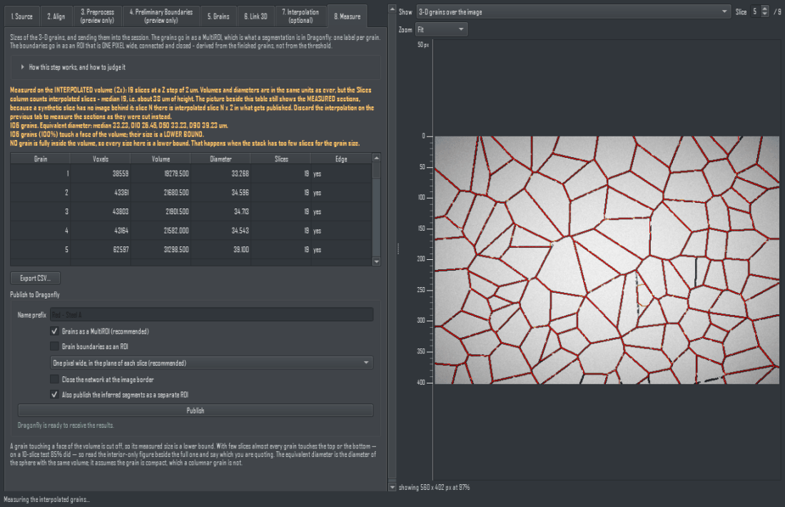
The Measure tab, shown with an interpolation in force: the first line is the interpolated banner, naming the factor and the Z step, and the Slices column counts interpolated slices. Below it, per-grain volume and equivalent diameter, the D10/D50/D90 spread, and how many grains touch a face of the volume — those are lower bounds.

A grain touching a face of the volume is cut off, so its measured size is a lower bound. With few slices almost every grain touches the top or the bottom - on a 10-slice test 85% did - so the interior-only mean is given beside the full one and you should say which you are quoting.

Publishing sends the grains in as a MultiROI, one label per grain named with its size, and optionally the boundary network as an ROI. Geometry is copied from the source channel, so the result sits exactly on the image it came from. Two more boxes, both on by default: Publish the aligned image as well puts the aligned, cropped grey image in beside the grains and the boundaries (only when the stack was aligned and not interpolated), and Grains that touch no face of the volume as a separate MultiROI adds a second MultiROI holding only the grains whose size is complete, renumbered consecutively, each label named after the grain's number in the table.

When an interpolation is in force, four things about publishing change. Every title gains (interpolated x8). The Z spacing written into the published objects is the section step divided by the factor - 0.0625 um instead of 0.5 um at 8x - so distances measured in Dragonfly are right (this override was verified in a running Dragonfly: a published MultiROI read back Z = 0.125 um against a 0.5 um source at 4x). The aligned grey image is not published alongside, because it has the measured stack's 40 slices against the labels' 313 and the two would not share a grid. And on an aligned stack, if Dragonfly refuses the shifted origin the publish fails with its reason instead of falling back to the source frame: that fallback undoes the per-slice whole-pixel shifts, and a synthetic slice has no shift of its own to undo.

The CSV holds every grain, plus two columns that record what was measured: slice_thickness, the Z step of the object the row came from, and source, which reads measured_sections or interpolated_x8. The suggested filename gains _interpolated_x8 for the same reason. Keep both columns when you paste the numbers into a report.

Publishing a slice sub-range is refused, with the reason: the new object inherits the source channel's origin and would land in the wrong place in Z. Load the full range, or export the CSV.

The boundary ROI: one pixel wide, connected, closed

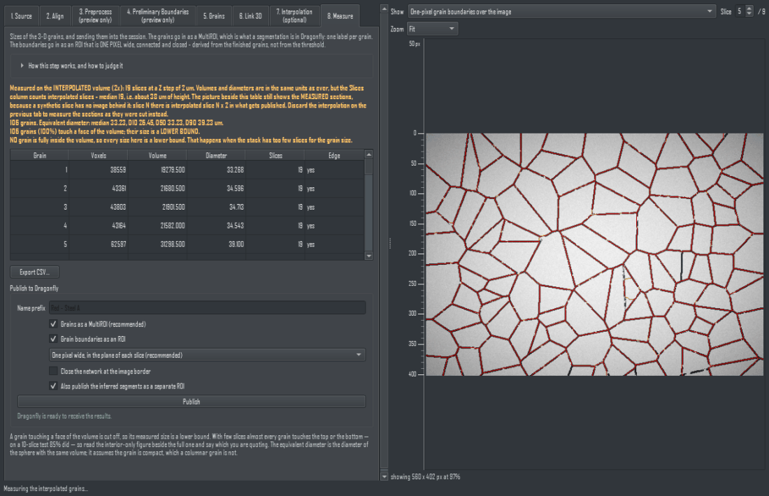
The boundary that gets published, shown over the image: one pixel wide, following the etched line where there is one and carrying straight on across the gaps where there is not, so no two grains are left touching.

The boundary that gets published is not the preliminary network from Tab 4. It is derived from the finished grains: for every pair of neighbouring grains a line is drawn between them, one pixel wide, whether or not the etch showed a line there. So two grains are always separated, the network never breaks, and you can trace it, measure its length, or use it as a mask.

The line is 8-connected and the grains it encloses are 4-connected - the standard pair, and the reason a diagonal step in the line does not leak. After publishing, the report states the size of the network, how many connected pieces it is in, and how many pixels (if any) could not be thinned to one. That last number should be zero; when it is not, it is a junction where four grains meet in a 2x2, which no one-pixel line can resolve - not a setting to tune.

• One pixel wide, in the plane of each slice is the recommended style and the default. On the reference data it is about 3% of the volume.
• Three-dimensional interface shell is the older reading: every voxel with a differently-labelled face neighbour, two voxels thick, 38% of the reference volume. It answers a different question, and on a stack of few slices it is close to meaningless.
• Close the network at the image border additionally paints the frame, so a grain cut by the edge of the field of view is enclosed too. Those pixels are not grain boundaries - leave the box unticked if you are going to measure boundary length.

A line pixel has to be taken from one of the two grains it separates, because on a pixel grid there is nowhere else to draw it. So the boundary ROI overlaps the grain MultiROI and the grains keep the sizes in the table; subtract the ROI from the MultiROI in Dragonfly if you need the two to be disjoint. To see the network before publishing, set the picture selector to Grain boundaries, one pixel wide - that is the very array Publish will hand over.

Supported and inferred line [2026-09-06] A line pixel is supported when an etched groove pixel of its own slice lies within 2 px of it; the rest of the line is inferred - it records where the 3-D flood decided two grains meet, with nothing in that slice's image to show for it (typically an under-etched slice). The complete one-pixel network is published as before; with Also publish the inferred segments as a separate ROI ticked (the default) the inferred part goes in as a second ROI whose title ends in inferred, the report states the supported share, and the preview Boundaries over the image: etched (green), inferred (magenta) shows the two on the picture. Not offered for an interpolated volume, whose synthetic slices have no image behind them.

10. How to tell whether your stack can be reconstructed at all

This is the question to settle before trusting any 3-D number, and the plugin answers it for you in the Tab 5 table.

• If most intervals show a median IoU around 0.6 or higher, the slices are close enough together and the grains can be tracked.
• If most intervals are low and most grains span one slice, the polishing removed about a grain's worth of material per step. No algorithm can fix that; the specimen has to be re-sectioned with a smaller step. As a rule of thumb, aim for at least five slices through the smallest grain you care about.
• A few isolated breaks in an otherwise good stack simply split it into blocks. Each block between two breaks is a valid 3-D volume; measure the blocks separately rather than reporting one number across a break.

11. What this plugin does not do

• It does not measure orientation, and nothing here can be turned into a misorientation, a twin identification or a pole figure. An etched micrograph carries no orientation.
• It does not do a full registration. Tab 2 corrects a whole-pixel translation per slice and nothing else: no rotation, no scaling, no sub-pixel shift, no elastic warping. For any of those, use Dragonfly's own Slice Registration first and come back afterwards.
• It does not do sub-pixel boundary localisation. A boundary is a voxel face.
• It does not separate phases or identify inclusions; the dark blobs an etch leaves are treated as boundary or as specks by size alone.
• It does not assume grains are compact. It reports the equivalent diameter, which does, so for a columnar structure read the volume and the slice span instead.

9. Meshing (optional). Turns the grains into triangle meshes that still TOUCH. One mesh is built for the whole polycrystal with SHARED vertices, so the face between two grains exists once and belongs to both; smoothing moves that one surface and both grains follow it. Meshing each grain on its own and smoothing it cannot do that - the surfaces drift apart by a fraction of a voxel everywhere - and neither can meshing the boundary ROI, whose one-voxel band comes back from marching cubes as a shell with two faces a voxel apart. Target voxel size defaults to the source image's own Z step, because the shape between two sections is inferred rather than measured: on the reference stack, meshing at the pixel size gave 76 million triangles of which 87% were horizontal walls between slices - the staircase itself - against 1.9 million at the Z step. Smoothing is Taubin by default (it keeps the volume; a plain Laplacian shrank the same grains by 2.5%), every vertex is held inside its own half-voxel cell, and vertices where three or four grains meet are restrained or pinned so triple lines and corners survive. The report states that every grain is closed with outward normals and how its volume compares with the voxel count it came from; the picture beside it draws the mesh where the current slice cuts it, over the image itself. Publish the polycrystal as one Mesh, publish grains one by one up to a limit, or export every grain as a binary STL - which is the way to get thousands of them out.